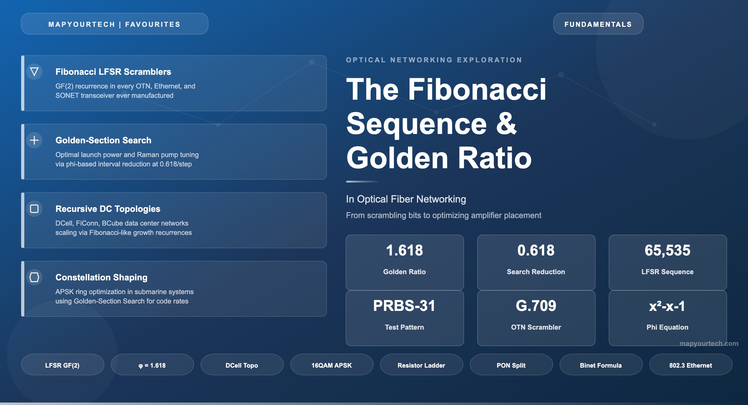
The Fibonacci Sequence and the Golden Ratio in Optical Fiber Networking
From scrambling bits to optimizing amplifier placement, from recursive data center topologies to constellation shaping — nature's favourite number shows up in surprising corners of photonic engineering.
Table of Contents
- 1. Introduction
- 2. The Fibonacci Sequence and Golden Ratio
- 3. Fibonacci LFSRs in Optical Scrambling
- 4. Golden-Section Search in Network Optimization
- 5. Recursive Topologies and Fibonacci Growth
- 6. The Shannon Limit, Capacity, and the Spiral
- 7. PON Splitting and Power Distribution
- 8. Amplifier Spacing and the Optimal Ratio
- 9. Resistor Ladders and the Golden Ratio
- 10. Summary of Connections
1. Introduction
The Fibonacci sequence — 0, 1, 1, 2, 3, 5, 8, 13, 21, 34, 55, 89, 144 ... — is one of the most recognized patterns in all of mathematics. Each number equals the sum of its two predecessors: Fn = Fn-1 + Fn-2. As the sequence progresses, the ratio of consecutive terms converges on the Golden Ratio, denoted φ (phi), which equals approximately 1.6180339887.
These mathematical structures appear everywhere in the natural world: the spiral of a nautilus shell, the branching of trees, the arrangement of petals in a sunflower. But they also appear — sometimes explicitly, sometimes in disguise — throughout the engineering disciplines that underpin modern optical fiber networking. This article maps those connections, separating genuine mathematical relationships from loose analogies, and showing where Fibonacci and φ serve real engineering purposes in photonic systems.
The connections range from the very direct (Fibonacci Linear Feedback Shift Registers used in every optical transceiver for bit scrambling) to the structural (recursive data center topologies that grow in Fibonacci-like patterns) to the mathematical (Golden-Section Search applied to optimize amplifier placement and launch power in DWDM links).
2. The Fibonacci Sequence and the Golden Ratio
Before exploring the connections to optical networking, it helps to establish the core mathematical properties that make these structures so useful in engineering.
The Fibonacci Recurrence: Fn = Fn-1 + Fn-2, with F0 = 0, F1 = 1.
The Golden Ratio: φ = (1 + √5) / 2 ≈ 1.6180339887...
The convergence: lim (Fn / Fn-1) = φ as n approaches infinity.
Self-similarity property: φ2 = φ + 1, and 1/φ = φ − 1 ≈ 0.618
2.1 Proof: Deriving φ from the Fibonacci Sequence
The claim that the ratio of consecutive Fibonacci numbers converges to the Golden Ratio is not something to take on faith. Here is a complete, step-by-step proof that derives the exact value φ = (1 + √5) / 2 directly from the Fibonacci recurrence.
Theorem: limn→∞ (Fn+1 / Fn) = (1 + √5) / 2
The Fibonacci sequence is defined by: Fn = Fn-1 + Fn-2, with F0 = 0, F1 = 1.
Write out the first several terms: 0, 1, 1, 2, 3, 5, 8, 13, 21, 34, 55, 89, 144, 233, 377 ...
Let rn = Fn+1 / Fn be the ratio of consecutive Fibonacci numbers. Compute a few values:
| n | Fn | Fn+1 | rn = Fn+1 / Fn | Error from φ |
|---|---|---|---|---|
| 1 | 1 | 1 | 1.000000 | 0.618034 |
| 2 | 1 | 2 | 2.000000 | 0.381966 |
| 3 | 2 | 3 | 1.500000 | 0.118034 |
| 4 | 3 | 5 | 1.666667 | 0.048633 |
| 5 | 5 | 8 | 1.600000 | 0.018034 |
| 6 | 8 | 13 | 1.625000 | 0.006966 |
| 7 | 13 | 21 | 1.615385 | 0.002649 |
| 8 | 21 | 34 | 1.619048 | 0.001014 |
| 9 | 34 | 55 | 1.617647 | 0.000387 |
| 10 | 55 | 89 | 1.618182 | 0.000148 |
| 15 | 610 | 987 | 1.618033 | 0.000001 |
| 20 | 6765 | 10946 | 1.618034 | < 10-8 |
Table: The ratio oscillates above and below φ, converging rapidly. By n = 15, the ratio matches φ to six decimal places.
Assume that rn converges to some limit L as n → ∞. That is:
limn→∞ Fn+1 / Fn = L
(The proof that this limit exists uses the monotone convergence theorem on alternating subsequences of rn — rn alternates above and below φ with decreasing amplitude, so both the odd-indexed and even-indexed subsequences converge, and they converge to the same value.)
Take the defining recurrence Fn+1 = Fn + Fn-1 and divide every term by Fn:
  Fn+1 / Fn  =  Fn / Fn  +  Fn-1 / Fn

  Simplifying:

  rn  =  1  +  1 / rn-1
This is the step where the magic happens. We have expressed the current ratio purely in terms of the previous ratio.
As n → ∞, both rn and rn-1 approach L. Substituting:
L = 1 + 1 / LThis single equation contains the entire derivation of the Golden Ratio.
Multiply both sides by L to eliminate the fraction:
  L2  =  L  +  1

  Rearranging to standard form:

  L2 − L − 1 = 0

  Apply the quadratic formula (a=1, b=−1, c=−1):

  L  =  (1 ± √(1 + 4)) / 2
L = (1 ± √5) / 2The two solutions are:
  L1 = (1 + √5) / 2  ≈  +1.6180339887...
  L2 = (1 − √5) / 2  ≈  −0.6180339887...
Since every Fibonacci number (for n ≥ 1) is positive, the ratio Fn+1 / Fn is always positive. Therefore L must be positive, and we discard L2.
limn→∞ Fn+1 / Fn = (1 + √5) / 2 = φ ≈ 1.6180339887...
The Golden Ratio emerges directly and necessarily from the Fibonacci recurrence. Any sequence defined by "each term equals the sum of the two before it" will produce ratios that converge to φ, regardless of the starting values (as long as both are positive).
2.2 The Self-Similarity Property: φ2 = φ + 1
Notice that the equation we solved in Step 6 — L2 = L + 1 — is itself the defining property of the Golden Ratio. This means φ is the unique positive number whose square equals itself plus one. This self-referential property makes φ appear anywhere a system exhibits recursive self-similarity: the whole relates to the larger part exactly as the larger part relates to the smaller.
Useful identities that follow from φ2 = φ + 1:
1/φ = φ − 1 ≈ 0.618034 — (the "reciprocal Golden Ratio" used in Golden-Section Search)
φ3 = φ2 × φ = (φ + 1) × φ = φ2 + φ = 2φ + 1 ≈ 4.236
φn = Fn × φ + Fn-1 — (every power of φ is a linear combination of φ and 1, with Fibonacci coefficients)
2.3 Visualizing the Convergence
The chart below shows how the ratio Fn+1/Fn oscillates above and below φ with rapidly decreasing amplitude. By n = 10, the ratio matches φ to three decimal places. By n = 20, the match extends to eight decimal places. This fast convergence is why φ appears so reliably in any system governed by a Fibonacci-type recurrence.
Figure: Convergence of Fn+1/Fn toward the Golden Ratio φ ≈ 1.618034. The oscillating approach from alternating sides is characteristic of this sequence.
2.4 Binet's Formula: The Closed-Form Expression
The value 0.618 (the reciprocal of φ) turns out to be just as important as φ itself. It is the ratio that drives the Golden-Section Search algorithm used in numerical optimization — a method directly applicable to optical network design problems. And Binet's closed-form formula gives us any Fibonacci number without recursion:
  Fn = (φn − ψn) / √5

  Where: φ = (1 + √5) / 2  ≈  1.618
         ψ = (1 − √5) / 2  ≈ −0.618
The self-similarity property (φ2 = φ + 1) means that any system built on φ-based ratios exhibits a kind of mathematical elegance: the whole relates to the larger part exactly as the larger part relates to the smaller. This property drives optimal interval reduction in search algorithms and underlies the efficient packing behaviour seen in everything from sunflower seeds to antenna arrays.
3. Fibonacci LFSRs in Optical Scrambling
This is the most direct and indisputable connection between the Fibonacci name and optical communications. Every modern optical transceiver, from 10G SFP+ modules to 800G ZR+ coherent transceivers, uses a Fibonacci-configuration Linear Feedback Shift Register (LFSR) for data scrambling.
3.1 What Problem Does Scrambling Solve?
In an optical transmission system, long runs of identical bits (all 1s or all 0s) create problems. A string of continuous 1s at a fixed amplitude contains no transitions for the receiver's clock and data recovery (CDR) circuit to lock onto. The receiver loses bit synchronization and errors cascade. Additionally, long repeated patterns create spectral lines — concentrated energy at specific frequencies — that can interfere with other channels in a DWDM system or violate the spectral emission masks defined by standards.
Scrambling solves both problems by XOR-combining the data stream with a pseudorandom binary sequence (PRBS) generated by a Fibonacci LFSR. The result looks statistically random to the receiver's CDR circuit while remaining perfectly deterministic and reversible. The same LFSR structure at the receiver (running the same polynomial) recovers the original data.
3.2 The Fibonacci LFSR Architecture
In a Fibonacci LFSR, a chain of flip-flops forms a shift register, and the outputs of selected positions (called taps) are fed through XOR gates back to the first register's input. The name "Fibonacci" comes from the recursive feedback structure: just as each Fibonacci number is the sum of two predecessors, each new bit in the register is a function of previous bits at specific positions.
The feedback connections are defined by a primitive polynomial over GF(2) (the Galois field with two elements, 0 and 1). For an n-bit Fibonacci LFSR with a properly chosen primitive polynomial, the register cycles through all 2n − 1 non-zero states before repeating, producing a maximal-length sequence (m-sequence).
  Practical Example: OTN Scrambler

  Polynomial:  x16 + x12 + x3 + x + 1
  Register length:  16 bits
  Sequence length:  216 − 1 = 65,535 bits before repeat
  Architecture:  Fibonacci (external XOR)

  Each clock cycle:
  input_bit = tap[16] XOR tap[12] XOR tap[3] XOR tap[1]
  All registers shift right by one position
The alternative architecture, called the Galois LFSR, places XOR gates between the register stages rather than feeding all taps to a single external XOR. The Galois configuration can operate at higher clock speeds because each XOR gate sees only two inputs (reducing propagation delay), but the Fibonacci configuration remains the standard reference form used in protocol specifications. IEEE 802.3 Ethernet, ITU-T G.709 OTN, and numerous other optical standards specify their scramblers and PRBS test patterns using Fibonacci LFSR polynomials.
Where Fibonacci LFSRs Appear
OTN frame scrambling (G.709), Ethernet 64B/66B encoding, SONET/SDH scramblers, PRBS test patterns (PRBS-7, PRBS-15, PRBS-31), spread-spectrum clock generation in transceivers, CRC calculation for error detection.
The Fibonacci Property in LFSRs
The m-sequence output has a balance property (number of 1s exceeds 0s by exactly one), a run property (runs of length k occur 2n−k−1 times), and near-ideal autocorrelation — properties that make it excellent for DC balance and spectral flatness in optical links.
4. Golden-Section Search in Network Optimization
The Golden-Section Search is a classical numerical optimization technique for finding the minimum (or maximum) of a unimodal function within a bounded interval. It narrows the search interval by a factor of 1/φ ≈ 0.618 at each step, making it the optimal fixed-ratio interval reduction method. The algorithm was first developed by Jack Kiefer in 1953 and is the continuous-domain limit of the Fibonacci search technique.
4.1 How It Works
Given an interval [a, b] and a function f(x) with a single minimum inside it, the algorithm evaluates f at two interior points that divide the interval in the Golden Ratio. By comparing the function values, one of the outer endpoints is discarded, and the interval shrinks by the factor φ − 1 ≈ 0.618. The elegance is that one of the two interior evaluation points from the previous iteration can always be reused, so only one new function evaluation is needed per iteration.
  Golden-Section Search: Interval Reduction

  r = φ − 1 ≈ 0.618
  c = 1 − r ≈ 0.382

  At each iteration, three interval widths maintain the ratio:
      φ : 1 : φ

  After n iterations, interval reduced by factor:
      rn = 0.618n

  Practical Example: To find optimum launch power within a 20 dB range
  to within 0.1 dB accuracy:
      n = ln(0.1/20) / ln(0.618) ≈ 11 iterations
4.2 Applications in Optical Network Design
Optical network optimization is full of unimodal functions that are expensive to evaluate. The per-channel launch power in a DWDM system, for instance, has a single optimum: too low and the signal drowns in amplified spontaneous emission (ASE) noise; too high and fiber nonlinearities (self-phase modulation, cross-phase modulation, four-wave mixing) degrade the signal. The OSNR-vs-power curve has a clear peak, making it an ideal candidate for Golden-Section Search.
Similarly, amplifier spacing optimization in long-haul and submarine systems produces a unimodal performance curve. Shorter spans mean more amplifiers (higher cost and more accumulated ASE), while longer spans mean higher per-span loss and lower OSNR. Analytical work on undersea transmission systems has shown that the optimum span length depends primarily on fiber loss coefficient α, with the relationship lopt = 2/α. Golden-Section Search provides an efficient numerical method to find this optimum when the analytical approximation is not precise enough for a given system configuration.
Other optical design problems suited to this method include: EDFA gain tilt optimization per channel, dispersion compensation ratio tuning, Raman pump power optimization, and flex-grid channel width selection for maximum aggregate throughput.
5. Recursive Topologies and Fibonacci Growth Patterns
Modern hyperscale data center networks use topologies that grow through recursion — building higher-level structures by connecting copies of lower-level building blocks. This mirrors the Fibonacci sequence's defining property: each new term is constructed from the two that came before it.
5.1 DCell Architecture
The DCell architecture, proposed for data center networks, builds its connectivity through a recursive construction. A DCell0 consists of a switch connected to a small number of servers. A DCell1 is built from multiple DCell0 units, where each server has an additional network interface connecting it to a server in a different DCell0. A DCell2 is built from multiple DCell1 units using the same principle. The number of servers at each level grows in a pattern that, while not identical to the Fibonacci sequence, follows the same recursive construction principle. If a DCell0 contains n servers, the total server count at level k is determined by the recurrence: tk = (tk-1 + 1) × tk-1, which produces hyper-exponential growth driven by recursive self-similarity.
5.2 FiConn: Fibonacci in the Name
A variant of DCell, explicitly called FiConn, limits each server to exactly two network interfaces and trades capacity and redundancy for lower cost and cabling complexity. The FiConn topology grows by connecting lower-level cells into higher-level cells, and the name itself references the Fibonacci-like recursive construction: each level builds on the previous two in a structured way, with the number of interconnections between levels following patterns related to Fibonacci growth.
5.3 BCube and Other Recursive Architectures
The BCube architecture follows a similar philosophy, adding switch layers recursively. Each level adds a new tier of switches connecting one server from each lower-level cell. These recursive data center topologies share a common mathematical DNA with the Fibonacci sequence: they define structure at level n in terms of structures at levels n−1 and n−2 (or lower), producing networks where the total element count, path diversity, and fault tolerance emerge from the recursive rule rather than from a fixed blueprint.
The Clos network architecture (originally proposed by Charles Clos in 1953 for telephone switching) also connects to this theme. The leaf-spine fabric used in nearly every modern data center is a two-level Clos network, and multi-level Clos networks expand recursively — a pattern that scales connectivity in a manner analogous to Fibonacci growth.
6. The Shannon Limit, Capacity, and the Spiral
Coherent optical systems transmit data by encoding information onto the amplitude and phase of a light wave. The received signal is represented as a point in the complex plane (the constellation diagram), and phase noise from the transmitter and local oscillator lasers causes these constellation points to rotate. When viewed over time, phase noise traces a spiral pattern in the I-Q plane that is mathematically related to logarithmic spirals — a class of curves intimately connected to the Golden Ratio.
6.1 Phase Noise and the Spiral
Laser phase noise is modelled as a Wiener process (random walk in phase). In a constellation diagram, this produces a gradual rotation of constellation points. When the accumulated phase drift is plotted against received signal magnitude over many symbols, the result is a smeared spiral pattern. The logarithmic spiral, also called the spira mirabilis (wonderful spiral), has the property that it looks the same at every scale — a self-similarity directly related to the Golden Ratio. While the phase noise spiral in coherent receivers is stochastic rather than deterministic, its statistical envelope follows the same mathematical family as the Golden Spiral.
6.2 Constellation Shaping and Fibonacci-Adjacent Optimization
Approaching Shannon's capacity limit on the fiber channel requires constellation shaping — adjusting either the geometry (geometric shaping) or the probability distribution (probabilistic shaping) of constellation points. In advanced undersea transmission systems, coded modulation formats like 4D-PS-56APSK use ring constellations where the radii of successive rings are optimized based on Gaussian distributions. The ratios of these ring radii from inner to outer (reported as 1 : 1.88 : 2.71 : 3.95 in experimental work on transoceanic systems) are the result of optimization procedures that often employ Golden-Section Search or Fibonacci search to find the optimal ring spacing that maximizes Euclidean distance between 4D constellation points.
The spectral efficiency range achievable with variable coded modulation — from 4.5 to 10.2 b/s/Hz using APSK-based formats — is tuned through inner code rate variation, and the search for optimal code rate combinations across wavelengths in a WDM system is itself an optimization problem where Golden-Section methods apply.
7. PON Splitting and Power Distribution
Passive Optical Networks (PONs) use optical splitters to distribute a single fiber's signal to multiple end users. The split ratio directly determines the power budget: each 1:2 split introduces approximately 3.5 dB of loss. The total loss for a 1:N split is approximately 10 × log10(N) dB plus excess losses.
  Split Ratio Power Loss:

  Loss(dB) = 10 × log10(N) + excess loss

  Common splits:  1:2  →  ~3.5 dB
                  1:4  →  ~7.0 dB
                  1:8  →  ~10.5 dB
                  1:16 →  ~13.5 dB
                  1:32 →  ~16.5 dB
                  1:64 →  ~19.5 dB
The commonly deployed split ratios — 1:2, 1:4, 1:8, 1:16, 1:32, 1:64 — all follow powers of 2 for practical manufacturing reasons. However, the question of optimal split ratio for a given link budget is itself a minimization problem: splitting too little wastes fiber plant (under-serves subscribers), while splitting too much drives the signal below receiver sensitivity. This optimization, constrained by discrete available splitter values, can be approached through Fibonacci search when the objective function (cost per subscriber, for instance) is unimodal over the range of candidate split ratios.
More interestingly, when designing hierarchical PON architectures with cascaded splitters (a 1:4 splitter feeding four 1:8 splitters, for example), the total loss budget at each branching level follows an additive progression in dB that parallels the summation property of the Fibonacci sequence — each level's loss is the sum of its own splitting loss plus the accumulated loss from all previous levels.
8. Amplifier Spacing and the Optimal Ratio
One of the most important optimization problems in long-haul and submarine optical system design is determining the optimal amplifier spacing. The relationship between amplifier spacing, spectral efficiency, and total link performance produces a curve with a clear optimum.
For EDFA-amplified systems, analytical work based on the Gaussian Noise (GN) model has established that the peak achievable spectral efficiency (SE) increases as amplifier spacing decreases — more amplifiers mean lower gain per amplifier, less ASE noise per amplifier, and therefore better OSNR. However, in power-constrained systems like submarine cables, the available electrical power limits the number of amplifiers that can be deployed. The optimum span length for maximum power efficiency has been derived analytically as lopt = 2/α, where α is the fiber loss coefficient in linear units per km.
For a standard G.652 fiber with 0.2 dB/km loss (or α ≈ 0.046/km in linear units), this gives lopt ≈ 43 km — which aligns well with the typical 40–50 km repeater spacing used in modern submarine cable systems. The fact that this optimum depends only on fiber loss and is independent of bandwidth, number of spatial dimensions, or amplifier noise figure is a remarkable simplification that mirrors the elegance of Golden Ratio mathematics — a single ratio governing system-wide performance.
When the analytical approximation is not precise enough (for example, in systems with hybrid Raman+EDFA amplification, or when nonlinear effects must be accounted for more carefully), numerical optimization using Golden-Section Search provides an efficient way to find the true optimum within the design space.
9. Resistor Ladders and the Golden Ratio in Photonic Circuits
A well-known result in electrical engineering, published in the American Journal of Physics, demonstrates that the effective resistance of an infinite ladder network of identical resistors equals the Golden Ratio times the resistance of a single resistor. This is because the infinite ladder satisfies the same self-similarity condition as φ: removing one rung from an infinite ladder leaves another infinite ladder, producing the equation Rtotal = R + R × Rtotal / (R + Rtotal), which resolves to Rtotal = φ × R.
This result has a photonic analogue. In silicon photonic circuits and integrated optical delay lines, cascaded Mach-Zehnder interferometer (MZI) stages form optical "ladder" networks. The transfer function of a cascade of identical MZI stages, when analysed using z-transform methods over GF(2), exhibits the same Fibonacci recurrence relation that governs LFSRs. The power coupling ratios in optimally designed cascaded MZI filters converge toward values related to the Golden Ratio, particularly when the design target is a maximally flat passband response.
The broader lesson is that any system where identical stages are cascaded and each stage's output feeds forward into the next carries the mathematical fingerprint of the Fibonacci sequence. In optical networking, this pattern appears in cascaded amplifier chains, multi-stage ROADM architectures, and concatenated FEC decoder iterations.
10. Summary of Connections
The following table consolidates the genuine connections between Fibonacci/Golden Ratio mathematics and optical fiber networking, rated by the directness of the mathematical relationship.
| Connection | Fibonacci / φ Role | Optical Networking Application | Strength |
|---|---|---|---|
| Fibonacci LFSR | Explicit — architecture named for Fibonacci recurrence | Scrambling in OTN, Ethernet, SONET; PRBS test patterns; CRC | Direct |
| Golden-Section Search | φ-based interval reduction for unimodal optimization | Launch power, amplifier gain, Raman pump power optimization | Direct |
| Fibonacci Search | Discrete Fibonacci-number interval reduction (precursor to Golden-Section) | Parameter sweep with limited function evaluations | Direct |
| Recursive DC Topologies | Fibonacci-like recurrence in node count growth | DCell, FiConn, BCube data center network scaling | Structural |
| Infinite Resistor Ladder | Effective resistance = φ × R | Cascaded MZI filter design, optical ladder networks | Analogous |
| Constellation Optimization | Golden-Section Search for ring radii, code rates | APSK ring spacing, variable SE optimization in submarine systems | Indirect |
| Phase Noise Spiral | Logarithmic spiral related to Golden Spiral | Phase noise visualization in coherent I-Q diagrams | Analogous |
| PON Split Optimization | Fibonacci/Golden-Section Search for optimal split ratio | Cost-per-subscriber minimization in FTTH deployments | Indirect |
Table 1: Summary of Fibonacci and Golden Ratio connections in optical networking, rated by mathematical directness.
Fibonacci Sequence Growth vs. Optical Capacity Growth
An interesting visual comparison: the Fibonacci sequence's growth rate (approaching φn / √5) closely mirrors the exponential growth trajectory of deployed optical fiber capacity over the decades. Both follow a roughly exponential envelope, though capacity growth is driven by engineering innovation rather than a pure mathematical recurrence.
Figure 1: Normalized growth comparison — Fibonacci sequence (mathematical) vs. representative optical capacity trajectory (engineering). Both exhibit exponential-class growth.
The Deeper Pattern
The Fibonacci sequence and the Golden Ratio are not merely curiosities that happen to appear in optical networking. They show up because they are fundamental to three classes of problems that optical engineers face daily: recursive construction (building large systems from repeated small units), optimal search (finding the best parameter value with minimal evaluations), and pseudorandom generation (creating sequences with ideal statistical properties for scrambling and testing).
The Fibonacci LFSR is perhaps the most ubiquitous mathematical construct in all of digital optical communications — present in every single transceiver ever manufactured, running continuously whenever light carries data through glass. The Golden-Section Search quietly optimizes the systems those transceivers operate in. And recursive topologies built on Fibonacci-like growth rules connect the servers that generate the traffic those systems carry.
Mathematics does not care whether it is describing sunflower seeds or DWDM channels. The same structures that produce natural beauty produce engineering efficiency — and in optical networking, Fibonacci and φ do exactly that.
References
- J. Kiefer, "Sequential Minimax Search for a Maximum," Proceedings of the American Mathematical Society.
- S. Kumar, G. Papen, K. Schmidtke, and C. Xie, "Intra-data Center Interconnects, Networking, and Architectures," Optical Fiber Telecommunications V11, Elsevier.
- C. Li, et al., "DCell: A Scalable and Fault-Tolerant Network Structure for Data Centers," ACM SIGCOMM.
- J.-Y. Cai et al., "On the Capacity of Undersea Transmission Systems with Variable Spectral Efficiency," Optical Fiber Telecommunications V11, Elsevier.
- P. Poggiolini et al., "The GN-model of Fiber Non-linear Propagation and Its Applications," Journal of Lightwave Technology.
- S. Somekh, "Fibonacci Sequence, Golden Ratio, and a Network of Resistors," American Journal of Physics.
- W.H. Press et al., "Golden Section Search in One Dimension," Numerical Recipes: The Art of Scientific Computing, Cambridge University Press.
- ITU-T G.709 — Interfaces for the Optical Transport Network, ITU-T Study Group 15.
Sanjay Yadav, "Optical Network Communications: An Engineer's Perspective" – Bridge the Gap Between Theory and Practice in Optical Networking.
Developed by MapYourTech Team
Note: This article is curated with the help of internet-based research, grounded in MapYourTech's personal interest and fascination with the Fibonacci sequence and the Golden Ratio. It is meant for appreciating how nature's mathematical patterns find their way into the engineering systems we build — from the geometry of photonic crystals to the algorithms inside optical transceivers. The connections presented here are drawn from published, peer-reviewed research; where a connection is speculative or absent from the literature, it is clearly noted.
Feedback Welcome: If you have any suggestions, corrections, or improvements to propose, please feel free to write to us at [email protected]

Optical Communications & Network Automation Expert | Author of 3 Books for Optical Engineers | Founder, MapYourTech
Optical networking engineer with nearly two decades of experience across DWDM, OTN, coherent optics, submarine systems, and cloud infrastructure. Founder of MapYourTech. Read full bio →
Follow on LinkedInRelated Articles on MapYourTech