


1. Introduction and Background
Optical networks form the backbone of modern communications infrastructure, enabling the high-speed transmission of vast amounts of data across global networks. While bandwidth has traditionally been the primary focus of network performance metrics, latency has emerged as an equally critical parameter, particularly for time-sensitive applications. Latency, defined as the delay from the time of packet transmission at the sender to the end of packet reception at the receiver, can significantly impact the overall performance of communication systems even when bandwidth remains constant.
The evolution of optical networking technologies has continually pushed the boundaries of data transmission capabilities. However, as applications become increasingly time-sensitive, the focus has shifted toward minimizing delay in addition to maximizing throughput. This shift represents a fundamental change in how we evaluate network performance and design optical communication systems.
Historically, optical networks were primarily designed to maximize bandwidth and transmission distance. The first-generation systems focused on basic point-to-point connections, while subsequent generations introduced wavelength division multiplexing (WDM) to increase capacity. Modern systems have evolved to include advanced techniques for dispersion compensation, signal amplification, and digital signal processing, all of which affect latency in various ways.
Key components contributing to latency in optical networks and potential optimization strategies
2. Fundamentals of Latency in Optical Systems
2.1 Physical Principles of Latency
At its most basic level, latency in optical fiber networks arises from the time it takes light to travel through the transmission medium. While light travels at approximately 299,792.458 km/s in vacuum, it propagates more slowly in optical fiber due to the refractive index of the material. This fundamental physical constraint establishes a lower bound on achievable latency.
The effective group index of refraction (neff) is a critical parameter that determines the actual speed of light in an optical fiber. It represents a weighted average of all the indices of refraction encountered by light as it travels within the fiber. For standard single-mode fiber (SMF) defined by ITU-T G.652 recommendation, the neff is approximately 1.4676 for transmission at 1310 nm and 1.4682 for transmission at 1550 nm wavelength.
Using these values, we can calculate the speed of light in optical fiber:
At 1310 nm wavelength: v₁₃₁₀ = c/neff = 299,792.458 km/s / 1.4676 = 204,271.5 km/s
At 1550 nm wavelength: v₁₅₅₀ = c/neff = 299,792.458 km/s / 1.4682 = 204,189.7 km/s
This translates to a propagation delay of approximately:
- 4.895 μs/km at 1310 nm
- 4.897 μs/km at 1550 nm
These values represent the theoretical minimum latency for signal transmission over optical fiber, assuming no additional delays from other network components or processing overhead.
2.2 Major Sources of Latency in Optical Networks
Beyond the inherent delay caused by light propagation in fiber, multiple components and processes contribute to the overall latency in optical networks. These can be broadly categorized into:
- Optical Fiber Delays:
- Propagation delay (approximately 4.9 μs/km)
- Additional delay due to fiber type and refractive index profile
- Optical Component Delays:
- Amplifiers (e.g., EDFAs add approximately 0.15 μs due to 30m of erbium-doped fiber)
- Dispersion compensation modules (DCMs)
- Fiber Bragg gratings (FBGs)
- Optical switches and ROADMs (Reconfigurable Optical Add-Drop Multiplexers)
- Opto-Electrical Component Delays:
- Transponders and muxponders (typically 5-10 μs per unit)
- O-E-O conversion (approximately 100 μs)
- Digital signal processing (up to 1 μs)
- Forward Error Correction (15-150 μs depending on algorithm)
- Protocol and Processing Delays:
- Higher OSI layer processing
- Data packing and unpacking
- Switching and routing decisions
Key Insight: Latency Sources and Contributions
The total end-to-end latency in an optical network is the sum of multiple delay components. While fiber propagation delay often constitutes the largest portion (60-80%), other components can add significant overhead. Understanding the relative contribution of each component is crucial for effective latency optimization.
3. Applications Requiring Low Latency
3.1 Financial Services
In the financial sector, particularly in high-frequency trading, latency can have a direct impact on profitability. Even a 10 ms delay can potentially result in a 10% drop in revenue. Modern trading systems have moved from executing transactions within seconds to requiring millisecond, microsecond, and now even nanosecond response times. Some institutions can complete transactions within 0.35 μs during high-frequency trading.
Key requirements:
- Ultra-low latency (sub-millisecond)
- High stability (minimal jitter)
- Predictable performance
3.2 Interactive Entertainment Services
Time-critical, bandwidth-hungry services such as 4K/8K video, virtual reality (VR), and augmented reality (AR) require low-latency networks to provide a seamless user experience. For VR services specifically, industry consensus suggests that latency should not exceed 20 ms to avoid vertigo and ensure a positive user experience.
Key requirements:
- Latency < 20 ms
- Consistent performance
- High bandwidth
3.3 IoT and Real-Time Cloud Services
Applications such as data hot backup, cloud desktop, and intra-city disaster recovery also benefit from low-latency networks. For optimal cloud desktop service experience and high-reliability intra-city data center disaster recovery, latency requirements are typically less than 20 ms.
Key requirements:
- Latency < 20 ms
- Reliability
- Scalability
3.4 5G and Autonomous Systems
Emerging technologies like autonomous driving require extremely low latency to function safely. For autonomous driving, the end-to-end latency requirement is approximately 5 ms, with a round-trip time (RTT) latency of 2 ms reserved for the transport network.
Key requirements:
- Latency < 1 ms
- Ultra-high reliability
- Widespread coverage
| Application | Maximum Acceptable Latency | One-Way/Round-Trip | Critical Factors | Recommended Technologies |
|---|---|---|---|---|
| High-Frequency Trading | 0.35-1 ms | One-way | • Consistency • Deterministic performance |
• Direct fiber routes • Hollow-core fiber • Minimal processing |
| Virtual/Augmented Reality | 20 ms | Round-trip | • Low jitter • Consistent performance |
• Edge computing • Optimized backbone • Content caching |
| Cloud Services | 20 ms | Round-trip | • Reliability • Scalability |
• Distributed data centers • Full-mesh topology • Protocol optimization |
| Autonomous Driving | 5 ms | Round-trip | • Ultrahigh reliability • Widespread coverage |
• Mobile edge computing • 5G integration • URLLC protocols |
| 5G URLLC Services | 1 ms | Round-trip | • Coverage • Reliability |
• Fiber fronthaul/backhaul • Distributed architecture |
4. Mathematical Models and Analysis
4.1 Propagation Delay Modeling
The propagation delay in optical fiber can be modeled mathematically as:
Delay (in seconds) = Length (in meters) / Velocity (in meters/second)Where velocity is determined by:
Velocity = c / neffWith c being the speed of light in vacuum (299,792,458 m/s) and neff being the effective group index of refraction.
For a fiber of length L with an effective group index of refraction neff, the propagation delay T can be calculated as:
T = L × neff / cThis equation forms the foundation for understanding latency in optical networks and serves as the starting point for more complex analysis involving additional network components.
4.2 Chromatic Dispersion Effects on Latency
Chromatic dispersion (CD) occurs because different wavelengths of light travel at different speeds in optical fiber. This not only causes signal distortion but also contributes to latency. The accumulated chromatic dispersion D in a fiber of length L can be calculated as:
D = Dfiber × LWhere Dfiber is the dispersion coefficient of the fiber (typically measured in ps/nm/km).
For standard single-mode fiber (SMF) with a dispersion coefficient of approximately 17 ps/nm/km at 1550 nm, a 100 km fiber link would accumulate about 1700 ps/nm of dispersion, requiring compensation to maintain signal quality.
4.3 Latency Budget Analysis
When designing low-latency optical networks, engineers often perform latency budget analysis to account for all sources of delay:
Total Latency = Tfiber + Tcomponents + Tprocessing + TFEC + TDSPWhere:
- Tfiber is the propagation delay in the fiber
- Tcomponents is the delay introduced by optical components
- Tprocessing is the delay from signal processing
- TFEC is the delay from forward error correction
- TDSP is the delay from digital signal processing
This comprehensive approach allows for precise latency calculations and helps identify opportunities for optimization.
5. Latency Optimization Strategies
| Component | Typical Latency | Percentage of Total Latency | Optimization Techniques | Latency Reduction Potential |
|---|---|---|---|---|
| Fiber Propagation | 4.9 µs/km | 60-80% | • Hollow-core fiber • Route optimization • Straight-line deployment |
Up to 31% |
| Amplification | 0.15 µs per EDFA | 1-3% | • Raman amplification • Minimizing amplifier count • Optimized EDFA design |
Up to 90% |
| Dispersion Compensation | 15-25% of fiber delay | 10-20% | • FBG instead of DCF • Coherent detection with DSP • Dispersion-shifted fiber |
95-99% |
| OEO Conversion | ~100 µs | 5-15% | • All-optical switching (ROADM/OXC) • Optimized transponders • Reducing conversion points |
Up to 100% (elimination) |
| Forward Error Correction | 15-150 µs | 5-20% | • Optimized FEC algorithms • Flexible FEC levels • Low-latency coding schemes |
50-90% |
| Protocol Processing | Variable (ns to ms) | 1-10% | • Lower OSI layer protocols • Protocol stack simplification • Hardware acceleration |
50-70% |
5.1 Route Optimization
One of the most direct approaches to reducing latency is optimizing the physical route of the optical fiber. This can involve:
- Deploying fiber along the shortest possible path between endpoints
- Simplifying network architecture to reduce forwarding nodes
- Constructing one-hop transmission networks to reduce system latency
- Optimizing conventional ring or chain topologies to full-mesh topologies during backbone network planning
Such optimizations reduce the physical distance light must travel, thereby minimizing propagation delay.
5.2 Fiber Type Selection
Different types of optical fibers offer varying latency characteristics:
- Standard Single-Mode Fiber (SMF, G.652): The most commonly deployed fiber type with neff of approximately 1.467-1.468.
- Non-Zero Dispersion-Shifted Fiber (NZ-DSF, G.655): Optimized for regional and metropolitan high-speed optical networks operating in the C- and L-optical bands. These fibers have lower chromatic dispersion (typically 2.6-6.0 ps/nm/km in C-band) than standard SMF, requiring simpler dispersion compensation that adds only up to 5% to the transmission time.
- Dispersion-Shifted Fiber (DSF, G.653): Optimized for use in the 1550 nm region with zero chromatic dispersion at 1550 nm wavelength, potentially eliminating the need for dispersion compensation. However, it’s limited to single-wavelength operation due to nonlinear effects like four-wave mixing (FWM).
- Photonic Crystal Fibers (PCFs): These specialty fibers can have very low effective refractive indices. Hollow-core fibers (HCFs), a type of PCF, may provide up to 31% reduced latency compared to traditional fibers. However, they typically have higher attenuation (3.3 dB/km compared to 0.2 dB/km for SMF at 1550 nm), though recent advances have achieved attenuations as low as 1.2 dB/km.
Selecting the appropriate fiber type based on specific application requirements can significantly reduce latency.
| Fiber Type | Effective Group Index | Propagation Delay | Attenuation (at 1550 nm) | Special Considerations | Best Use Cases |
|---|---|---|---|---|---|
| Standard SMF (G.652) | ~1.4682 | 4.9 µs/km | 0.2 dB/km | • Widely deployed • Cost-effective |
• General purpose • Long-haul with DCM |
| NZ-DSF (G.655) | ~1.47 | 4.9 µs/km | 0.2 dB/km | • Lower dispersion • Simpler compensation |
• Regional networks • Metropolitan areas |
| DSF (G.653) | ~1.47 | 4.9 µs/km | 0.2 dB/km | • Zero dispersion at 1550 nm • FWM limitations |
• Single-wavelength • Point-to-point |
| Hollow-Core Fiber | 1.01-1.2 | 3.4-4.0 µs/km | 1.2-3.3 dB/km | • Higher attenuation • Specialized connectors |
• Ultra-low latency • Short critical links |
| Multi-Core Fiber | ~1.46-1.47 | 4.9 µs/km | 0.2 dB/km | • Higher capacity • Complex termination |
• High capacity • Space-constrained routes |
5.3 Optical-Layer Optimization
Several techniques can be employed at the optical layer to minimize latency:
- Coherent Communication Technology: Leveraging coherent detection eliminates the need for dispersion compensation fibers (DCFs), reducing latency. However, it introduces additional digital signal processing that can add up to 1 μs of delay.
- Fiber Bragg Grating (FBG) for Dispersion Compensation: Replacing DCF-based dispersion compensation modules with FBG-based ones can significantly reduce latency. While DCF adds 15-25% to the fiber propagation time, FBG typically introduces only 5-50 ns of delay.
- ROADM/OXC Implementation: Using Reconfigurable Optical Add-Drop Multiplexers (ROADM) and Optical Cross-Connects (OXC) enables optical-layer pass-through and switching, reducing the number of optical-electrical-optical (OEO) conversions.
- Raman Amplification: Replacing erbium-doped fiber amplifiers (EDFAs) with Raman amplifiers eliminates the need for erbium-doped fibers, avoiding the extra latency they introduce (typically 0.15 μs for 30m of erbium-doped fiber). Raman amplifiers also effectively extend all-optical transmission distances, reducing the need for electrical regeneration.
5.4 Electrical-Layer Optimization
At the electrical layer, several strategies can be employed to reduce latency:
- FEC Algorithm Optimization: Optimizing Forward Error Correction (FEC) algorithms can increase transmission distance while reducing latency penalties. Some systems allow flexible setting of FEC levels to balance error correction capability against latency.
- Transponder Selection: Simpler transponders without FEC or in-band management channels can operate at much lower latencies (4-30 ns compared to 5-10 μs for more complex units). Some vendors claim transponders operating with as little as 2 ns latency.
- Minimizing OEO Conversion: Avoiding optical-electrical-optical (OEO) conversion, which typically adds about 100 μs of latency, is crucial for low-latency networks.
- Flexible Service Encapsulation: Optimizing the service encapsulation mode can reduce processing overhead and associated latency.
5.5 Protocol Optimization
Network protocols significantly impact latency. WDM/OTN technologies operate at the physical (L0) and data link (L1) layers of the OSI model, offering the lowest possible latency:
- Lower OSI Layers: Protocols operating at lower OSI layers (L0/L1) introduce less latency (nanosecond level) compared to higher layers like L3/L4 (millisecond to hundreds of milliseconds).
- Protocol Simplification: Simplifying protocol stacks from 5 layers to 2 layers can reduce single-site latency by up to 70%.
- WDM/OTN Adoption: WDM/OTN technology provides latency close to the physical limit, with most latency coming from fiber transmission rather than protocol processing.
Key Insight: End-to-End Optimization
The most effective latency reduction strategies address multiple components in the optical network chain. For ultra-low latency applications like high-frequency trading, every microsecond matters, and optimizations must consider the entire path from end to end, including physical routes, component selection, and protocol implementation.6. Practical Implementation and Recommendations
| Component | Typical Implementation | Latency | Optimized Implementation | Latency | Reduction |
|---|---|---|---|---|---|
| Fiber (100 km) | Standard SMF | 490 µs | Hollow-core fiber | 338 µs | 31% |
| Amplifiers | 2 EDFAs | 0.3 µs | 1 Raman amplifier | 0 µs | 100% |
| Dispersion Compensation | DCF modules | 98 µs | FBG-based or coherent | 0.05 µs | 99.9% |
| Transponders | Standard with FEC | 10 µs | Low-latency specialized | 0.03 µs | 99.7% |
| OEO Conversion | 1 regeneration point | 100 µs | All-optical path | 0 µs | 100% |
| Protocol Processing | Multiple OSI layers | 5 µs | L0/L1 only | 0.5 µs | 90% |
| Total End-to-End | 703.3 µs | 338.58 µs | 51.9% |
6.1 Network Architecture Design
When designing low-latency optical networks, consider the following architectural principles:
- Direct Connectivity: Implement direct fiber connections between critical nodes rather than routing through intermediate points.
- Mesh Topology: Adopt a mesh topology rather than ring or chain topologies to minimize hop count between endpoints.
- Physical Route Planning: Carefully plan fiber routes to minimize physical distance, even if it means higher initial deployment costs.
- Redundancy with Latency Awareness: Design redundant paths with similar latency characteristics to maintain consistent performance during failover events.
6.2 Component Selection Guidelines
Select network components based on their latency characteristics:
- Fiber Selection:
- Use hollow-core or photonic crystal fibers for ultra-low-latency requirements where budget permits
- Consider NZ-DSF (G.655) for metropolitan networks to reduce dispersion compensation needs
- Amplification:
- Prefer Raman amplification over EDFA where possible
- If using EDFA, select designs with minimal erbium-doped fiber length
- Dispersion Compensation:
- Choose FBG-based compensation over DCF-based solutions
- For ultra-low-latency applications, consider coherent detection with electrical dispersion compensation, weighing the DSP latency against DCF latency
- Transponders and Muxponders:
- Select simple transponders without unnecessary functionality for critical low-latency paths
- Consider latency-optimized transponders (some vendors offer units with 2-30 ns latency)
- Evaluate the trade-off between FEC capability and latency impact
6.3 Management and Monitoring
Implementing effective latency management and monitoring is crucial:
- Latency SLA Definition: Clearly define latency Service Level Agreements (SLAs) for different application requirements.
- Threshold Monitoring: Implement latency threshold crossing and jitter alarm functions to detect when service latency exceeds predefined thresholds.
- Dynamic Routing: Utilize latency optimization functions to reroute services whose latency exceeds thresholds, ensuring committed SLAs are maintained.
- Regular Testing: Perform regular latency tests and measurements to identify degradation or opportunities for improvement.
- End-to-End Visibility: Implement monitoring tools that provide visibility into all components contributing to latency.
6.4 Industry-Specific Implementations
Different industries have unique latency requirements and implementation considerations:
- Financial Services:
- Deploy dedicated, physical point-to-point dark fiber connections between trading facilities
- Minimize or eliminate intermediate equipment
- Consider hollow-core fiber for critical routes despite higher cost
- Implement precision timing and synchronization
- Interactive Entertainment:
- Focus on consistent latency rather than absolute minimum values
- Implement edge computing to bring resources closer to users
- Design for peak load conditions to avoid latency spikes
- IoT and Cloud Services:
- Distribute data centers strategically to minimize distance to end users
- Implement intelligent caching and content delivery networks
- Optimize for both latency and jitter
- 5G and Autonomous Systems:
- Design for ultra-reliable low latency communication (URLLC)
- Implement mobile edge computing (MEC) to minimize backhaul latency
- Ensure comprehensive coverage to maintain consistent performance
7. Future Trends and Research Directions
7.1 Advanced Fiber Technologies
Research into novel fiber designs continues to push the boundaries of latency reduction:
- Next-Generation Hollow-Core Fibers: Improvements in hollow-core fiber design are reducing attenuation while maintaining the latency advantage. Research aims to achieve attenuation values closer to standard SMF while providing 30-40% latency reduction.
- Multi-Core and Few-Mode Fibers: Although primarily developed for capacity enhancement, these fibers might offer latency advantages through spatial mode management.
- Engineered Refractive Index Profiles: Custom-designed refractive index profiles could optimize for both latency and other transmission characteristics.
7.2 Integrated Photonics
The miniaturization and integration of optical components promise significant latency reductions:
- Silicon Photonics: Integration of multiple optical functions onto silicon chips can reduce physical distances between components and minimize latency.
- Photonic Integrated Circuits (PICs): These offer the potential to replace multiple discrete components with a single integrated device, reducing both physical size and signal propagation time.
- Co-packaged Optics: Bringing optical interfaces closer to electronic switches and routers reduces the need for electrical traces and interconnects, potentially lowering latency.
7.3 Machine Learning for Latency Optimization
Artificial intelligence and machine learning techniques are being applied to latency optimization:
- Predictive Routing: ML algorithms can predict network conditions and optimize routes based on expected latency performance.
- Dynamic Resource Allocation: Intelligent systems can allocate network resources based on application latency requirements and current network conditions.
- Anomaly Detection: ML can identify latency anomalies and potential issues before they impact service quality.
7.4 Quantum Communications
Quantum technologies may eventually offer novel approaches to latency reduction:
- Quantum Entanglement: While not breaking the speed-of-light limit, quantum entanglement could potentially enable new communication protocols with different latency characteristics.
- Quantum Repeaters: These could extend the reach of quantum networks without the latency penalties associated with classical regeneration.
8. Conclusion
Latency in optical networks represents a complex interplay of physical constraints, component characteristics, and processing overhead. As applications become increasingly sensitive to delay, understanding and optimizing these factors becomes crucial for network designers and operators.
The fundamental limits imposed by the speed of light in optical fiber establish a baseline for latency that cannot be overcome without changing the transmission medium itself. However, significant improvements can be achieved through careful route planning, fiber selection, component optimization, and protocol design.
Different applications have varying latency requirements, from the sub-microsecond demands of high-frequency trading to the more moderate needs of cloud services. Meeting these diverse requirements requires a tailored approach that considers the specific characteristics and priorities of each use case.
Looking forward, advances in fiber technology, integrated photonics, machine learning, and potentially quantum communications promise to push the boundaries of what’s possible in low-latency optical networking. As research continues and technology evolves, we can expect further reductions in latency and improvements in network performance.
For network operators and service providers, the ability to deliver low and predictable latency will increasingly become a competitive differentiator. Those who can provide networks with lower and more stable latency will gain advantages in business competition across multiple industries, from finance to entertainment, cloud computing, and beyond.
9. References
- ITU-T G.652 – Characteristics of a single-mode optical fibre and cable
- ITU-T G.653 – Characteristics of a dispersion-shifted single-mode optical fibre and cable
- ITU-T G.655 – Characteristics of a non-zero dispersion-shifted single-mode optical fibre and cable
- Poletti, F., et al. “Towards high-capacity fibre-optic communications at the speed of light in vacuum.” Nature Photonics 7, 279–284 (2013).
- Feuer, M.D., et al. “Joint Digital Signal Processing Receivers for Spatial Superchannels.” IEEE Photonics Technology Letters 24, 1957-1960 (2012).
- Layec, P., et al. “Low Latency FEC for Optical Communications.” Journal of Lightwave Technology 37, 3643-3654 (2019).
- MapYourTech, “Latency in Fiber Optic Networks,” 2025.
- Optical Internetworking Forum (OIF), “Implementation Agreement for CFP2-Analog Coherent Optics Module” (2018).
- “LATENCY IN OPTICAL TRANSMISSION NETWORKS 101,” 2025.
- Savory, S.J. “Digital Coherent Optical Receivers: Algorithms and Subsystems.” IEEE Journal of Selected Topics in Quantum Electronics 16, 1164-1179 (2010).
- Winzer, P.J. “High-Spectral-Efficiency Optical Modulation Formats.” Journal of Lightwave Technology 30, 3824-3835 (2012).
- Ip, E., et al. “Coherent detection in optical fiber systems.” Optics Express 16, 753-791 (2008).
- Agrawal, G.P. “Fiber-Optic Communication Systems,” 4th Edition, Wiley (2010).
- Richardson, D.J., et al. “Space-division multiplexing in optical fibres.” Nature Photonics 7, 354–362 (2013).
- Kikuchi, K. “Fundamentals of Coherent Optical Fiber Communications.” Journal of Lightwave Technology 34, 157-179 (2016).

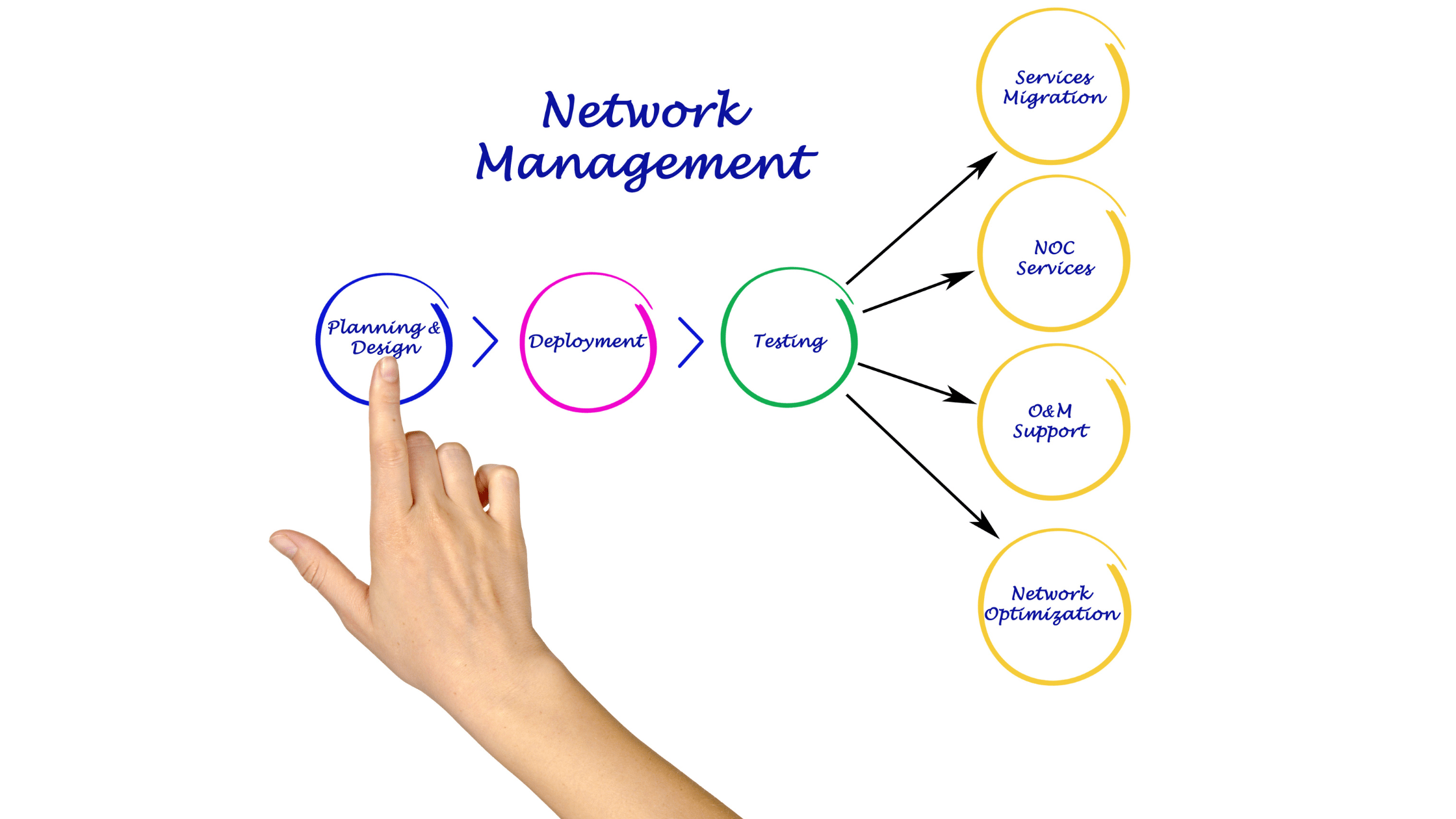
Network Management is crucial for maintaining the performance, reliability, and security of modern communication networks. With the rapid growth of network scales—from small networks with a handful of Network Elements (NEs) to complex infrastructures comprising millions of NEs—selecting the appropriate management systems and protocols becomes essential. Lets delves into the multifaceted aspects of network management, emphasizing optical networks and networking device management systems. It explores the best practices and tools suitable for varying network scales, integrates context from all layers of network management, and provides practical examples to guide network administrators in the era of automation.
1. Introduction to Network Management
Network Management encompasses a wide range of activities and processes aimed at ensuring that network infrastructure operates efficiently, reliably, and securely. It involves the administration, operation, maintenance, and provisioning of network resources. Effective network management is pivotal for minimizing downtime, optimizing performance, and ensuring compliance with service-level agreements (SLAs).
Key functions of network management include:
- Configuration Management: Setting up and maintaining network device configurations.
- Fault Management: Detecting, isolating, and resolving network issues.
- Performance Management: Monitoring and optimizing network performance.
- Security Management: Protecting the network from unauthorized access and threats.
- Accounting Management: Tracking network resource usage for billing and auditing.
In modern networks, especially optical networks, the complexity and scale demand advanced management systems and protocols to handle diverse and high-volume data efficiently.
2. Importance of Network Management in Optical Networks
Optical networks, such as Dense Wavelength Division Multiplexing (DWDM) and Optical Transport Networks (OTN), form the backbone of global communication infrastructures, providing high-capacity, long-distance data transmission. Effective network management in optical networks is critical for several reasons:
- High Throughput and Low Latency: Optical networks handle vast amounts of data with minimal delay, necessitating precise management to maintain performance.
- Fault Tolerance: Ensuring quick detection and resolution of faults to minimize downtime is vital for maintaining service reliability.
- Scalability: As demand grows, optical networks must scale efficiently, requiring robust management systems to handle increased complexity.
- Resource Optimization: Efficiently managing wavelengths, channels, and transponders to maximize network capacity and performance.
- Quality of Service (QoS): Maintaining optimal signal integrity and minimizing bit error rates (BER) through careful monitoring and adjustments.
Managing optical networks involves specialized protocols and tools tailored to handle the unique characteristics of optical transmission, such as signal power levels, wavelength allocations, and fiber optic health metrics.
3. Network Management Layers
Network management can be conceptualized through various layers, each addressing different aspects of managing and operating a network. This layered approach helps in organizing management functions systematically.
3.1. Lifecycle Management (LCM)
Lifecycle Management oversees the entire lifecycle of network devices—from procurement and installation to maintenance and decommissioning. It ensures that devices are appropriately managed throughout their operational lifespan.
- Procurement: Selecting and acquiring network devices.
- Installation: Deploying devices and integrating them into the network.
- Maintenance: Regular updates, patches, and hardware replacements.
- Decommissioning: Safely retiring old devices from the network.
Example: In an optical network, LCM ensures that new DWDM transponders are integrated seamlessly, firmware is kept up-to-date, and outdated transponders are safely removed.
3.2. Network Service Management (NSM)
Network Service Management focuses on managing the services provided by the network. It includes the provisioning, configuration, and monitoring of network services to meet user requirements.
- Service Provisioning: Allocating resources and configuring services like VLANs, MPLS, or optical channels.
- Service Assurance: Monitoring service performance and ensuring SLAs are met.
- Service Optimization: Adjusting configurations to optimize service quality and resource usage.
Example: Managing optical channels in a DWDM system to ensure that each channel operates within its designated wavelength and power parameters to maintain high data throughput.
3.3. Element Management Systems (EMS)
Element Management Systems are responsible for managing individual network elements (NEs) such as routers, switches, and optical transponders. EMS handles device-specific configurations, monitoring, and fault management.
- Device Configuration: Setting up device parameters and features.
- Monitoring: Collecting device metrics and health information.
- Fault Management: Detecting and addressing device-specific issues.
Example: An EMS for a DWDM system manages each optical transponder’s settings, monitors signal strength, and alerts operators to any deviations from normal parameters.
3.4. Business Support Systems (BSS)
Business Support Systems interface the network with business processes. They handle aspects like billing, customer relationship management (CRM), and service provisioning from a business perspective.
- Billing and Accounting: Tracking resource usage for billing purposes.
- CRM Integration: Managing customer information and service requests.
- Service Order Management: Handling service orders and provisioning.
Example: BSS integrates with network management systems to automate billing based on the optical channel usage in an OTN setup, ensuring accurate and timely invoicing.
3.5. Software-Defined Networking (SDN) Orchestrators and Controllers
SDN Orchestrators and Controllers provide centralized management and automation capabilities, decoupling the control plane from the data plane. They enable dynamic network configuration and real-time adjustments based on network conditions.
- SDN Controller: Manages the network’s control plane, making decisions about data flow and configurations.
- SDN Orchestrator: Coordinates multiple controllers and automates complex workflows across the network.
![]()
Image Credit: Wiki
Example: In an optical network, an SDN orchestrator can dynamically adjust wavelength allocations in response to real-time traffic demands, optimizing network performance and resource utilization.
4. Network Management Protocols and Standards
Effective network management relies on various protocols and standards designed to facilitate communication between management systems and network devices. This section explores key protocols, their functionalities, and relevant standards.
4.1. SNMP (Simple Network Management Protocol)
SNMP is one of the oldest and most widely used network management protocols, primarily for monitoring and managing network devices.
- Versions: SNMPv1, SNMPv2c, SNMPv3
- Standards:
- RFC 1157: SNMPv1
- RFC 1905: SNMPv2
- RFC 3411-3418: SNMPv3
Key Features:
- Monitoring: Collection of device metrics (e.g., CPU usage, interface status).
- Configuration: Basic configuration through SNMP SET operations.
- Trap Messages: Devices can send unsolicited alerts (traps) to managers.
Advantages:
- Simplicity: Easy to implement and use for basic monitoring.
- Wide Adoption: Supported by virtually all network devices.
- Low Overhead: Lightweight protocol suitable for simple tasks.
Disadvantages:
- Security: SNMPv1 and SNMPv2c lack robust security features. SNMPv3 addresses this but is more complex.
- Limited Functionality: Primarily designed for monitoring, with limited configuration capabilities.
- Scalability Issues: Polling large numbers of devices can generate significant network traffic.
Use Cases:
- Small to medium-sized networks for basic monitoring and alerting.
- Legacy systems where advanced management protocols are not supported.
4.2. NETCONF (Network Configuration Protocol)
NETCONF is a modern network management protocol designed to provide a standardized way to configure and manage network devices.
- Version: NETCONF v1.1
- Standards:
- RFC 6241: NETCONF Protocol
- RFC 6242: NETCONF over TLS
Key Features:
- Structured Configuration: Uses XML/YANG data models for precise configuration.
- Transactional Operations: Supports atomic commits and rollbacks to ensure configuration integrity.
- Extensibility: Modular and extensible, allowing for customization and new feature integration.
Advantages:
- Granular Control: Detailed configuration capabilities through YANG models.
- Transaction Support: Ensures consistent configuration changes with commit and rollback features.
- Secure: Typically operates over SSH or TLS, providing strong security.
Disadvantages:
- Complexity: Requires understanding of YANG data models and XML.
- Resource Intensive: Can be more demanding in terms of processing and bandwidth compared to SNMP.
Use Cases:
- Medium to large-sized networks requiring precise configuration and management.
- Environments where transactional integrity and security are paramount.
4.3. RESTCONF
RESTCONF is a RESTful API-based protocol that builds upon NETCONF principles, providing a simpler and more accessible interface for network management.
- Version: RESTCONF v1.0
- Standards:
- RFC 8040: RESTCONF Protocol
Key Features:
- RESTful Architecture: Utilizes standard HTTP methods (GET, POST, PUT, DELETE) for network management.
- Data Formats: Supports JSON and XML, making it compatible with modern web applications.
- YANG Integration: Uses YANG data models for defining network configurations and states.
Advantages:
- Ease of Use: Familiar RESTful API design makes it easier for developers to integrate with web-based tools.
- Flexibility: Can be easily integrated with various automation and orchestration platforms.
- Lightweight: Less overhead compared to NETCONF’s XML-based communication.
Disadvantages:
- Limited Transaction Support: Does not inherently support transactional operations like NETCONF.
- Security Complexity: While secure over HTTPS, integrating with OAuth or other authentication mechanisms can add complexity.
Use Cases:
- Environments where integration with web-based applications and automation tools is required.
- Networks that benefit from RESTful interfaces for easier programmability and accessibility.
4.4. gNMI (gRPC Network Management Interface)
gNMI is a high-performance network management protocol designed for real-time telemetry and configuration management, particularly suitable for large-scale and dynamic networks.
- Version: gNMI v0.7.x
- Standards: OpenConfig standard for gNMI
Key Features:
- Streaming Telemetry: Supports real-time, continuous data streaming from devices to management systems.
- gRPC-Based: Utilizes the efficient gRPC framework over HTTP/2 for low-latency communication.
- YANG Integration: Leverages YANG data models for consistent configuration and telemetry data.
Advantages:
- Real-Time Monitoring: Enables high-frequency, real-time data collection for performance monitoring and fault detection.
- Efficiency: Optimized for high throughput and low latency, making it ideal for large-scale networks.
- Automation-Friendly: Easily integrates with modern automation frameworks and tools.
Disadvantages:
- Complexity: Requires familiarity with gRPC, YANG, and modern networking concepts.
- Infrastructure Requirements: Requires scalable telemetry collectors and robust backend systems to handle high-volume data streams.
Use Cases:
- Large-scale networks requiring real-time performance monitoring and dynamic configuration.
- Environments that leverage software-defined networking (SDN) and network automation.
4.5. TL1 (Transaction Language 1)
TL1 is a legacy network management protocol widely used in telecom networks, particularly for managing optical network elements.
- Standards:
- Telcordia GR-833-CORE
- ITU-T G.773
- Versions: Varies by vendor/implementation
Key Features:
- Command-Based Interface: Uses structured text commands for managing network devices.
- Manual and Scripted Management: Supports both interactive command input and automated scripting.
- Vendor-Specific Extensions: Often includes proprietary commands tailored to specific device functionalities.
Advantages:
- Simplicity: Easy to learn and use for operators familiar with CLI-based management.
- Wide Adoption in Telecom: Supported by many legacy optical and telecom devices.
- Granular Control: Allows detailed configuration and monitoring of individual network elements.
Disadvantages:
- Limited Automation: Lacks the advanced automation capabilities of modern protocols.
- Proprietary Nature: Vendor-specific commands can lead to compatibility issues across different devices.
- No Real-Time Telemetry: Designed primarily for manual or scripted command entry without native support for continuous data streaming.
Use Cases:
- Legacy telecom and optical networks where TL1 is the standard management protocol.
- Environments requiring detailed, device-specific configurations that are not available through modern protocols.
4.6. CLI (Command Line Interface)
CLI is a fundamental method for managing network devices, providing direct access to device configurations and status through text-based commands.
- Standards: Vendor-specific, no universal standard.
- Versions: Varies by vendor (e.g., Cisco IOS, Juniper Junos, Huawei VRP)
Key Features:
- Text-Based Commands: Allows direct manipulation of device configurations through structured commands.
- Interactive and Scripted Use: Can be used interactively or automated using scripts.
- Universal Availability: Present on virtually all network devices, including routers, switches, and optical equipment.
Advantages:
- Flexibility: Offers detailed and granular control over device configurations.
- Speed: Allows quick execution of commands, especially for power users familiar with the syntax.
- Universality: Supported across all major networking vendors, ensuring broad applicability.
Disadvantages:
- Steep Learning Curve: Requires familiarity with specific command syntax and vendor-specific nuances.
- Error-Prone: Manual command entry increases the risk of human errors, which can lead to misconfigurations.
- Limited Scalability: Managing large numbers of devices through CLI can be time-consuming and inefficient compared to automated protocols.
Use Cases:
- Manual configuration and troubleshooting of network devices.
- Environments where precise, low-level device management is required.
- Small to medium-sized networks where automation is limited or not essential.
4.7. OpenConfig
OpenConfig is an open-source, vendor-neutral initiative designed to standardize network device configurations and telemetry data across different vendors.
- Standards: OpenConfig models are community-driven and continuously evolving.
- Versions: Continuously updated YANG-based models.
Key Features:
- Vendor Neutrality: Standardizes configurations and telemetry across multi-vendor environments.
- YANG-Based Models: Uses standardized YANG models for consistent data structures.
- Supports Modern Protocols: Integrates seamlessly with NETCONF, RESTCONF, and gNMI for configuration and telemetry.
Advantages:
- Interoperability: Facilitates unified management across diverse network devices from different vendors.
- Scalability: Designed to handle large-scale networks with automated management capabilities.
- Extensibility: Modular and adaptable to evolving network technologies and requirements.
Disadvantages:
- Adoption Rate: Not all vendors fully support OpenConfig models, limiting its applicability in mixed environments.
- Complexity: Requires understanding of YANG and modern network management protocols.
- Continuous Evolution: As an open-source initiative, models are frequently updated, necessitating ongoing adaptation.
Use Cases:
- Multi-vendor network environments seeking standardized management practices.
- Large-scale, automated networks leveraging modern protocols like gNMI and NETCONF.
- Organizations aiming to future-proof their network management strategies with adaptable and extensible models.
4.8. Syslog
Syslog is a standard for message logging, widely used for monitoring and troubleshooting network devices by capturing event messages.
- Version: Defined by RFC 5424
- Standards:
- RFC 3164: Original Syslog Protocol
- RFC 5424: Syslog Protocol (Enhanced)
Key Features:
- Event Logging: Captures and sends log messages from network devices to a centralized Syslog server.
- Severity Levels: Categorizes logs based on severity, from informational messages to critical alerts.
- Facility Codes: Identifies the source or type of the log message (e.g., kernel, user-level, security).
Advantages:
- Simplicity: Easy to implement and supported by virtually all network devices.
- Centralized Logging: Facilitates the aggregation and analysis of logs from multiple devices in one location.
- Real-Time Alerts: Enables immediate notification of critical events and issues.
Disadvantages:
- Unstructured Data: Traditional Syslog messages can be unstructured and vary by vendor, complicating log analysis.
- Reliability: UDP-based Syslog can result in message loss; however, TCP-based or Syslog over TLS solutions mitigate this issue.
- Scalability: Handling large volumes of log data requires robust Syslog servers and storage solutions.
Use Cases:
- Centralized monitoring and logging of network and optical devices.
- Real-time alerting and notification systems for network faults and security incidents.
- Compliance auditing and forensic analysis through aggregated log data.
5. Network Management Systems (NMS) and Tools
Network Management Systems (NMS) are comprehensive platforms that integrate various network management protocols and tools to provide centralized control, monitoring, and configuration capabilities. The choice of NMS depends on the scale of the network, specific requirements, and the level of automation desired.
5.1. For Small Networks (10 NEs)
Best Tools:
- PRTG Network Monitor: User-friendly, supports SNMP, Syslog, and other protocols. Ideal for small networks with basic monitoring needs.
- Nagios Core: Open-source, highly customizable, supports SNMP and Syslog. Suitable for administrators comfortable with configuring open-source tools.
- SolarWinds Network Performance Monitor (NPM): Provides a simple setup with powerful monitoring capabilities. Ideal for small to medium networks.
- Element Management System from any optical/networking vendor.
Features:
- Basic monitoring of device status, interface metrics, and uptime.
- Simple alerting mechanisms for critical events.
- Easy configuration with minimal setup complexity.
Example:
A small office network with a few routers, switches, and an optical transponder can use PRTG to monitor interface statuses, CPU usage, and power levels of optical devices via SNMP and Syslog.
5.2. For Medium Networks (100 NEs)
Best Tools:
- SolarWinds NPM: Scales well with medium-sized networks, offering advanced monitoring, alerting, and reporting features.
- Zabbix: Open-source, highly scalable, supports SNMP, NETCONF, RESTCONF, and gNMI. Suitable for environments requiring robust customization.
- Cisco Prime Infrastructure: Integrates seamlessly with Cisco devices, providing comprehensive management for medium-sized networks.
- Element Management System from any optical/networking vendor.
Features:
- Advanced monitoring with support for multiple protocols (SNMP, NETCONF).
- Enhanced alerting and notification systems.
- Configuration management and change tracking capabilities.
Example:
A medium-sized enterprise with multiple DWDM systems, routers, and switches can use Zabbix to monitor real-time performance metrics, configure devices via NETCONF, and receive alerts through Syslog messages.
5.3. For Large Networks (1,000 NEs)
Best Tools:
- Cisco DNA Center: Comprehensive management platform for large Cisco-based networks, offering automation, assurance, and advanced analytics.
- Juniper Junos Space: Scalable EMS for managing large Juniper networks, supporting automation and real-time monitoring.
- OpenNMS: Open-source, highly scalable, supports SNMP, RESTCONF, and gNMI. Suitable for diverse network environments.
- Network Management System from any optical/networking vendor.
Features:
- Centralized management with support for multiple protocols.
- High scalability and performance monitoring.
- Advanced automation and orchestration capabilities.
- Integration with SDN controllers and orchestration tools.
Example:
A large telecom provider managing thousands of optical transponders, DWDM channels, and networking devices can use Cisco DNA Center to automate configuration deployments, monitor network health in real-time, and optimize resource utilization through integrated SDN features.
5.4. For Enterprise and Massive Networks (500,000 to 1 Million NEs)
Best Tools:
- Ribbon LightSoft :Comprehensive network management solution for large-scale optical and IP networks.
- Nokia Network Services Platform (NSP): Highly scalable platform designed for massive network deployments, supporting multi-vendor environments.
- Huawei iManager U2000: Comprehensive network management solution for large-scale optical and IP networks.
- Splunk Enterprise: Advanced log management and analytics platform, suitable for handling vast amounts of Syslog data.
- Elastic Stack (ELK): Open-source solution for log aggregation, visualization, and analysis, ideal for massive log data volumes.
Features:
- Extreme scalability to handle millions of NEs.
- Advanced data analytics and machine learning for predictive maintenance and anomaly detection.
- Comprehensive automation and orchestration to manage complex network configurations.
- High-availability and disaster recovery capabilities.
Example:
A global internet service provider with a network spanning multiple continents, comprising millions of NEs including optical transponders, routers, switches, and data centers, can use Nokia NSP integrated with Splunk for real-time monitoring, automated configuration management through OpenConfig and gNMI, and advanced analytics to predict and prevent network failures.
6. Automation in Network Management
Automation in network management refers to the use of software tools and scripts to perform repetitive tasks, configure devices, monitor network performance, and respond to network events without manual intervention. Automation enhances efficiency, reduces errors, and allows network administrators to focus on more strategic activities.
6.1. Benefits of Automation
- Efficiency: Automates routine tasks, saving time and reducing manual workload.
- Consistency: Ensures uniform configuration and management across all network devices, minimizing discrepancies.
- Speed: Accelerates deployment of configurations and updates, enabling rapid scaling.
- Error Reduction: Minimizes human errors associated with manual configurations and monitoring.
- Scalability: Facilitates management of large-scale networks by handling complex tasks programmatically.
- Real-Time Responsiveness: Enables real-time monitoring and automated responses to network events and anomalies.
6.2. Automation Tools and Frameworks
- Ansible: Open-source automation tool that uses playbooks (YAML scripts) for automating device configurations and management tasks.
- Terraform: Infrastructure as Code (IaC) tool that automates the provisioning and management of network infrastructure.
- Python Scripts: Custom scripts leveraging libraries like Netmiko, Paramiko, and ncclient for automating CLI and NETCONF-based tasks.
- Cisco DNA Center Automation: Provides built-in automation capabilities for Cisco networks, including zero-touch provisioning and policy-based management.
- Juniper Automation: Junos Space Automation provides tools for automating complex network tasks in Juniper environments.
- Ribbon Muse SDN orchestrator ,Cisco MDSO and Ciena MCP/BluePlanet from any optical/networking vendor.
Example:
Using Ansible to automate the configuration of multiple DWDM transponders across different vendors by leveraging OpenConfig YANG models and NETCONF protocols ensures consistent and error-free deployments.
7. Best Practices for Network Management
Implementing effective network management requires adherence to best practices that ensure the network operates smoothly, efficiently, and securely.
7.1. Standardize Management Protocols
- Use Unified Protocols: Standardize on protocols like NETCONF, RESTCONF, and OpenConfig for configuration and management to ensure interoperability across multi-vendor environments.
- Adopt Secure Protocols: Always use secure transport protocols (SSH, TLS) to protect management communications.
7.2. Implement Centralized Management Systems
- Centralized Control: Use centralized NMS platforms to manage and monitor all network elements from a single interface.
- Data Aggregation: Aggregate logs and telemetry data in centralized repositories for comprehensive analysis and reporting.
7.3. Automate Routine Tasks
- Configuration Automation: Automate device configurations using scripts or automation tools to ensure consistency and reduce manual errors.
- Automated Monitoring and Alerts: Set up automated monitoring and alerting systems to detect and respond to network issues in real-time.
7.4. Maintain Accurate Documentation
- Configuration Records: Keep detailed records of all device configurations and changes for troubleshooting and auditing purposes.
- Network Diagrams: Maintain up-to-date network topology diagrams to visualize device relationships and connectivity.
7.5. Regularly Update and Patch Devices
- Firmware Updates: Regularly update device firmware to patch vulnerabilities and improve performance.
- Configuration Backups: Schedule regular backups of device configurations to ensure quick recovery in case of failures.
7.6. Implement Role-Based Access Control (RBAC)
- Access Management: Define roles and permissions to restrict access to network management systems based on job responsibilities.
- Audit Trails: Maintain logs of all management actions for security auditing and compliance.
7.7. Leverage Advanced Analytics and Machine Learning
- Predictive Maintenance: Use analytics to predict and prevent network failures before they occur.
- Anomaly Detection: Implement machine learning algorithms to detect unusual patterns and potential security threats.
8. Case Studies and Examples
8.1. Small Network Example (10 NEs)
Scenario: A small office network with 5 routers, 3 switches, and 2 optical transponders.
Solution: Use PRTG Network Monitor to monitor device statuses via SNMP and receive alerts through Syslog.
Steps:
- Setup PRTG: Install PRTG on a central server.
- Configure Devices: Enable SNMP and Syslog on all network devices.
- Add Devices to PRTG: Use SNMP credentials to add routers, switches, and optical transponders to PRTG.
- Create Alerts: Configure alerting thresholds for critical metrics like interface status and optical power levels.
- Monitor Dashboard: Use PRTG’s dashboard to visualize network health and receive real-time notifications of issues.
Outcome: The small network gains visibility into device performance and receives timely alerts for any disruptions, ensuring minimal downtime.
8.2. Optical Network Example
Scenario: A regional optical network with 100 optical transponders and multiple DWDM systems.
Solution: Implement OpenNMS with gNMI support for real-time telemetry and NETCONF for device configuration.
Steps:
- Deploy OpenNMS: Set up OpenNMS as the centralized network management platform.
- Enable gNMI and NETCONF: Configure all optical transponders to support gNMI and NETCONF protocols.
- Integrate OpenConfig Models: Use OpenConfig YANG models to standardize configurations across different vendors’ optical devices.
- Set Up Telemetry Streams: Configure gNMI subscriptions to stream real-time data on optical power levels and channel performance.
- Automate Configurations: Use OpenNMS’s automation capabilities to deploy and manage configurations across the optical network.
Outcome: The optical network benefits from real-time monitoring, automated configuration management, and standardized management practices, enhancing performance and reliability.
8.3. Enterprise Network Example
Scenario: A large enterprise with 10,000 network devices, including routers, switches, optical transponders, and data center equipment.
Solution: Utilize Cisco DNA Center integrated with Splunk for comprehensive management and analytics.
Steps:
- Deploy Cisco DNA Center: Set up Cisco DNA Center to manage all Cisco network devices.
- Integrate Non-Cisco Devices: Use OpenNMS to manage non-Cisco devices via NETCONF and gNMI.
- Setup Splunk: Configure Splunk to aggregate Syslog messages and telemetry data from all network devices.
- Automate Configuration Deployments: Use DNA Center’s automation features to deploy configurations and updates across thousands of devices.
- Implement Advanced Analytics: Use Splunk’s analytics capabilities to monitor network performance, detect anomalies, and generate actionable insights.
Outcome: The enterprise network achieves high levels of automation, real-time monitoring, and comprehensive analytics, ensuring optimal performance and quick resolution of issues.
9. Summary
Network Management is the cornerstone of reliable and high-performing communication networks, particularly in the realm of optical networks where precision and scalability are paramount. As networks continue to expand in size and complexity, the integration of advanced management protocols and automation tools becomes increasingly critical. By understanding and leveraging the appropriate network management protocols—such as SNMP, NETCONF, RESTCONF, gNMI, TL1, CLI, OpenConfig, and Syslog—network administrators can ensure efficient operation, rapid issue resolution, and seamless scalability.Embracing automation and standardization through tools like Ansible, Terraform, and modern network management systems (NMS) enables organizations to manage large-scale networks with minimal manual intervention, enhancing both efficiency and reliability. Additionally, adopting best practices, such as centralized management, standardized protocols, and advanced analytics, ensures that network infrastructures can meet the demands of the digital age, providing robust, secure, and high-performance connectivity.
Reference
- https://en.wikipedia.org/wiki/Software-defined_networking
- https://www.itu.int/rec/T-REC-M.3400-200002-I/en
- www.google.com
")
GUI (Graphical User Interface) interfaces have become a crucial part of network management systems, providing users with an intuitive, user-friendly way to manage, monitor, and configure network devices. Many modern networking vendors offer GUI-based management platforms, which are often referred to as Network Management Systems (NMS) or Element Management Systems (EMS), to simplify and streamline network operations, especially for less technically-inclined users or environments where ease of use is a priority.Lets explores the advantages and disadvantages of using GUI interfaces in network operations, configuration, deployment, and monitoring, with a focus on their role in managing networking devices such as routers, switches, and optical devices like DWDM and OTN systems.
Overview of GUI Interfaces in Networking
A GUI interface for network management typically provides users with a visual dashboard where they can manage network elements (NEs) through buttons, menus, and graphical representations of network topologies. Common tasks such as configuring interfaces, monitoring traffic, and deploying updates are presented in a structured, accessible way that minimizes the need for deep command-line knowledge.
Examples of GUI-based platforms include:
- Ribbons Muse, LighSoft
- Ciena One Control
- Cisco DNA Center for Cisco devices.
- Juniper’s Junos Space.
- Huawei iManager U2000 for optical and IP devices.
- Nokia Network Services Platform (NSP).
- SolarWinds Network Performance Monitor (NPM).
Advantages of GUI Interfaces
Ease of Use
The most significant advantage of GUI interfaces is their ease of use. GUIs provide a user-friendly and intuitive interface that simplifies complex network management tasks. With features such as drag-and-drop configurations, drop-down menus, and tooltips, GUIs make it easier for users to manage the network without needing in-depth knowledge of CLI commands.
- Simplified Configuration: GUI interfaces guide users through network configuration with visual prompts and wizards, reducing the chance of misconfigurations and errors.
- Point-and-Click Operations: Instead of remembering and typing detailed commands, users can perform most tasks using simple mouse clicks and menu selections.
This makes GUI-based management systems especially valuable for:
- Less experienced administrators who may not be familiar with CLI syntax.
- Small businesses or environments where IT resources are limited, and administrators need an easy way to manage devices without deep technical expertise.
Visualization of Network Topology
GUI interfaces often include network topology maps that provide a visual representation of the network. This feature helps administrators understand how devices are connected, monitor the health of the network, and troubleshoot issues quickly.
- Real-Time Monitoring: Many GUI systems allow real-time tracking of network status. Colors or symbols (e.g., green for healthy, red for failure) indicate the status of devices and links.
- Interactive Dashboards: Users can click on devices within the topology map to retrieve detailed statistics or configure those devices, simplifying network monitoring and management.
For optical networks, this visualization can be especially useful for managing complex DWDM or OTN systems where channels, wavelengths, and nodes can be hard to track through CLI.
Reduced Learning Curve
For network administrators who are new to networking or have limited exposure to CLI, a GUI interface reduces the learning curve. Instead of memorizing command syntax, users interact with a more intuitive interface that walks them through network operations step-by-step.
- Guided Workflows: GUI interfaces often provide wizards or guided workflows that simplify complex processes like device onboarding, VLAN configuration, or traffic shaping.
This can also speed up training for new IT staff, making it easier for them to get productive faster.
Error Reduction
In a GUI, configurations are typically validated on the fly, reducing the risk of syntax errors or misconfigurations that are common in a CLI environment. Many GUIs incorporate error-checking mechanisms, preventing users from making incorrect configurations by providing immediate feedback if a configuration is invalid.
- Validation Alerts: If a configuration is incorrect or incomplete, the GUI can generate alerts, prompting the user to fix the error before applying changes.
This feature is particularly useful when managing optical networks where incorrect channel configurations or power levels can cause serious issues like signal degradation or link failure.
Faster Deployment for Routine Tasks
For routine network operations such as firmware upgrades, device reboots, or creating backups, a GUI simplifies and speeds up the process. Many network management GUIs include batch processing capabilities, allowing users to:
- Upgrade the firmware on multiple devices simultaneously.
- Schedule backups of device configurations.
- Automate routine maintenance tasks with a few clicks.
For network administrators managing large deployments, this batch processing reduces the time and effort required to keep the network updated and functioning optimally.
Integrated Monitoring and Alerting
GUI-based network management platforms often come with built-in monitoring and alerting systems. Administrators can receive real-time notifications about network status, alarms, bandwidth usage, and device performance, all from a centralized dashboard. Some GUIs also integrate logging systems to help with diagnostics.
- Threshold-Based Alerts: GUI systems allow users to set thresholds (e.g., CPU utilization, link capacity) that, when exceeded, trigger alerts via email, SMS, or in-dashboard notifications.
- Pre-Integrated Monitoring Tools: Many GUI systems come with built-in monitoring capabilities, such as NetFlow analysis, allowing users to track traffic patterns and troubleshoot bandwidth issues.
Disadvantages of GUI Interfaces
Limited Flexibility and Granularity
While GUIs are great for simplifying network management, they often lack the flexibility and granularity of CLI. GUI interfaces tend to offer a subset of the full configuration options available through CLI. Advanced configurations or fine-tuning specific parameters may not be possible through the GUI, forcing administrators to revert to the CLI for complex tasks.
- Limited Features: Some advanced network features or vendor-specific configurations are not exposed in the GUI, requiring manual CLI intervention.
- Simplification Leads to Less Control: In highly complex network environments, some administrators may find that the simplification of GUIs limits their ability to make precise adjustments.
For example, in an optical network, fine-tuning wavelength allocation or optical channel power levels may be better handled through CLI or other specialized interfaces, rather than through a GUI, which may not support detailed settings.
Slower Operations for Power Users
Experienced network engineers often find GUIs slower to operate than CLI when managing large networks. CLI commands can be scripted or entered quickly in rapid succession, whereas GUI interfaces require more time-consuming interactions (clicking, navigating menus, waiting for page loads, etc.).
- Lag and Delays: GUI systems can experience latency, especially when managing a large number of devices, whereas CLI operations typically run with minimal lag.
- Reduced Efficiency for Experts: For network administrators comfortable with CLI, GUIs may slow down their workflow. Tasks that take a few seconds in CLI can take longer due to the extra navigation required in GUIs.
Resource Intensive
GUI interfaces are typically more resource-intensive than CLI. They require more computing power, memory, and network bandwidth to function effectively. This can be problematic in large-scale networks or when managing devices over low-bandwidth connections.
- System Requirements: GUIs often require more robust management servers to handle the graphical load and data processing, which increases the operational cost.
- Higher Bandwidth Use: Some GUI management systems generate more network traffic due to the frequent updates required to refresh the graphical display.
Dependence on External Management Platforms
GUI systems often require an external management platform (such as Cisco’s DNA Center or Juniper’s Junos Space), meaning they can’t be used directly on the devices themselves. This adds a layer of complexity and dependency, as the management platform must be properly configured and maintained.
- Single Point of Failure: If the management platform goes down, the GUI may become unavailable, forcing administrators to revert to CLI or other tools for device management.
- Compatibility Issues: Not all network devices, especially older legacy systems, are compatible with GUI-based management platforms, making it difficult to manage mixed-vendor or mixed-generation environments.
Security Vulnerabilities
GUI systems often come with more potential security risks compared to CLI. GUIs may expose more services (e.g., web servers, APIs) that could be exploited if not properly secured.
- Browser Vulnerabilities: Since many GUI systems are web-based, they can be susceptible to browser-based vulnerabilities, such as cross-site scripting (XSS) or man-in-the-middle (MITM) attacks.
- Authentication Risks: Improperly configured access controls on GUI platforms can expose network management to unauthorized users. GUIs tend to use more open interfaces (like HTTPS) than CLI’s more restrictive SSH.
Comparison of GUI vs. CLI for Network Operations
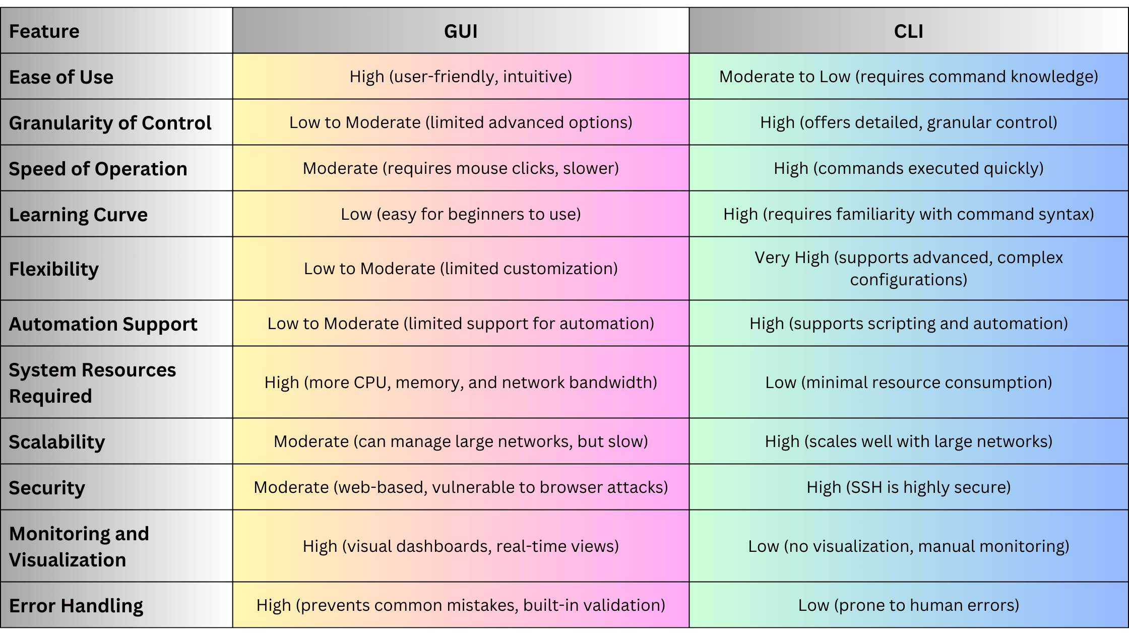
When to Use GUI Interfaces
GUI interfaces are ideal in the following scenarios:
- Small to Medium-Sized Networks: Where ease of use and simplicity are more important than advanced configuration capabilities.
- Less Technical Environments: Where network administrators may not have deep knowledge of CLI and need a simple, visual way to manage devices.
- Monitoring and Visualization: For environments where real-time network status and visual topology maps are needed for decision-making.
- Routine Maintenance and Monitoring: GUIs are ideal for routine tasks such as firmware upgrades, device status checks, or performance monitoring without requiring CLI expertise.
When Not to Use GUI Interfaces
GUI interfaces may not be the best choice in the following situations:
- Large-Scale or Complex Networks: Where scalability, automation, and fine-grained control are critical, CLI or programmable interfaces like NETCONF and gNMI are better suited.
- Time-Sensitive Operations: For power users who need to configure or troubleshoot devices quickly, CLI provides faster, more direct access.
- Advanced Configuration: For advanced configurations or environments where vendor-specific commands are required, CLI offers greater flexibility and access to all features of the device.
Summary
GUI interfaces are a valuable tool in network management, especially for less-experienced users or environments where ease of use, visualization, and real-time monitoring are priorities. They simplify network management tasks by offering an intuitive, graphical approach, reducing human errors, and providing real-time feedback. However, GUI interfaces come with limitations, such as reduced flexibility, slower operation, and higher resource requirements. As networks grow in complexity and scale, administrators may need to rely more on CLI, NETCONF, or gNMI for advanced configurations, scalability, and automation.
")
CLI (Command Line Interface) remains one of the most widely used methods for managing and configuring network and optical devices. Network engineers and administrators often rely on CLI to interact directly with devices such as routers, switches, DWDM systems, and optical transponders. Despite the rise of modern programmable interfaces like NETCONF, gNMI, and RESTCONF, CLI continues to be the go-to method for many due to its simplicity, direct access, and universal availability across a wide variety of network hardware.Let explore the fundamentals of CLI, its role in managing networking and optical devices, its advantages and disadvantages, and how it compares to other protocols like TL1, NETCONF, and gNMI. We will also provide practical examples of how CLI can be used to manage optical networks and traditional network devices.
What Is CLI?
CLI (Command Line Interface) is a text-based interface used to interact with network devices. It allows administrators to send commands directly to network devices, view status information, modify configurations, and troubleshoot issues. CLI is widely used in networking devices like routers and switches, as well as optical devices such as DWDM systems and Optical Transport Network (OTN) equipment.
Key Features:
- Text-Based Interface: CLI provides a human-readable way to manage devices by typing commands.
- Direct Access: Users connect to network devices through terminal applications like PuTTY or SSH clients and enter commands directly.
- Wide Support: Almost every networking and optical device from vendors like Ribbon, Ciena, Cisco, Juniper, Nokia, and others has a CLI.
- Manual or Scripted Interaction: CLI can be used both for manual configurations and scripted automation using tools like Python or Expect.
CLI is often the primary interface available for:
- Initial device configuration.
- Network troubleshooting.
- Monitoring device health and performance.
- Modifying network topologies.
CLI Command Structure
CLI commands vary between vendors but follow a general structure where a command invokes a specific action, and parameters or arguments are passed to refine the action. CLI commands can range from basic tasks, like viewing the status of an interface, to complex configurations of optical channels or advanced routing features.
Example of a Basic CLI Command (Cisco):
show ip interface briefThis command displays a summary of the status of all interfaces on a Cisco device.
Example of a CLI Command for Optical Devices:
show interfaces optical-1/1/1 transceiverThis command retrieves detailed information about the optical transceiver installed on interface optical-1/1/1, including power levels, wavelength, and temperature.
CLI Commands for Network and Optical Devices
Basic Network Device Commands
Show Commands
These commands provide information about the current state of the device. For example:
- show running-config: Displays the current configuration of the device.
- show ip route: Shows the routing table, which defines how packets are routed.
- show interfaces: Displays information about each network interface, including IP address, status (up/down), and traffic statistics.
Configuration Commands
Configuration mode commands allow you to make changes to the device’s settings.
- interface GigabitEthernet 0/1: Enter the configuration mode for a specific interface.
- ip address 192.168.1.1 255.255.255.0: Assign an IP address to an interface.
- no shutdown: Bring an interface up (enable it).
Optical Device Commands
Optical devices, such as DWDM systems and OTNs, often use CLI to monitor and manage optical parameters, channels, and alarms.
Show Optical Transceiver Status
Retrieves detailed information about an optical transceiver, including power levels and signal health.
show interfaces optical-1/1/1 transceiverSet Optical Power Levels
Configures the power output of an optical port to ensure the signal is within the required limits for transmission.
interface optical-1/1/1 transceiver power 0.0Monitor DWDM Channels
Shows the status and health of DWDM channels.
show dwdm channel-statusMonitor Alarms
Displays alarms related to optical devices, which can help identify issues such as low signal levels or hardware failures.
show alarmsCLI in Optical Networks
CLI plays a crucial role in optical network management, especially in legacy systems where modern APIs like NETCONF or gNMI may not be available. CLI is still widely used in DWDM systems, SONET/SDH devices, and OTN networks for tasks such as:
Provisioning Optical Channels
Provisioning optical channels on a DWDM system requires configuring frequency, power levels, and other key parameters using CLI commands. For example:
configure terminal
interface optical-1/1/1
  wavelength 1550.12
  transceiver power -3.5
  no shutdown
This command sequence configures optical interface 1/1/1 with a wavelength of 1550.12 nm and a power output of -3.5 dBm, then brings the interface online.
Monitoring Optical Performance
Using CLI, network administrators can retrieve performance data for optical channels and transceivers, including signal levels, bit error rates (BER), and latency.
show interfaces optical-1/1/1 transceiverThis retrieves key metrics for the specified optical interface, such as receive and transmit power levels, SNR (Signal-to-Noise Ratio), and wavelength.
Troubleshooting Optical Alarms
Optical networks generate alarms when there are issues such as power degradation, link failures, or hardware malfunctions. CLI allows operators to view and clear alarms:
show alarms
clear alarms
CLI Advantages
Simplicity and Familiarity
CLI has been around for decades and is deeply ingrained in the daily workflow of network engineers. Its commands are human-readable and simple to learn, making it a widely adopted interface for managing devices.
Direct Device Access
CLI provides direct access to network and optical devices, allowing engineers to issue commands in real-time without the need for additional layers of abstraction.
Universally Supported
CLI is supported across almost all networking devices, from routers and switches to DWDM systems and optical transponders. Vendors like Cisco, Juniper, Ciena, Ribbon, and Nokia all provide CLI access, making it a universal tool for network and optical management.
Flexibility
CLI can be used interactively or scripted using automation tools like Python, Ansible, or Expect. This makes it suitable for both manual troubleshooting and basic automation tasks.
Granular Control
CLI allows for highly granular control over network devices. Operators can configure specific parameters down to the port or channel level, monitor detailed statistics, and fine-tune settings.
CLI Disadvantages
Lack of Automation and Scalability
While CLI can be scripted for automation, it lacks the inherent scalability and automation features provided by modern protocols like NETCONF and gNMI. CLI does not support transactional operations or large-scale configuration changes easily.
Error-Prone
Because CLI is manually driven, there is a higher likelihood of human error when issuing commands. A misconfigured parameter or incorrect command can lead to service disruptions or device failures.
Vendor-Specific Commands
Each vendor often has its own set of CLI commands, which means that operators working with multiple vendors must learn and manage different command structures. For example, Cisco CLI differs from Juniper or Huawei CLI.
Limited Real-Time Data
CLI does not support real-time telemetry natively. It relies on manually querying devices or running scripts to retrieve data, which can miss crucial performance information or changes in network state.
CLI vs. Modern Protocols (NETCONF, gNMI, TL1)
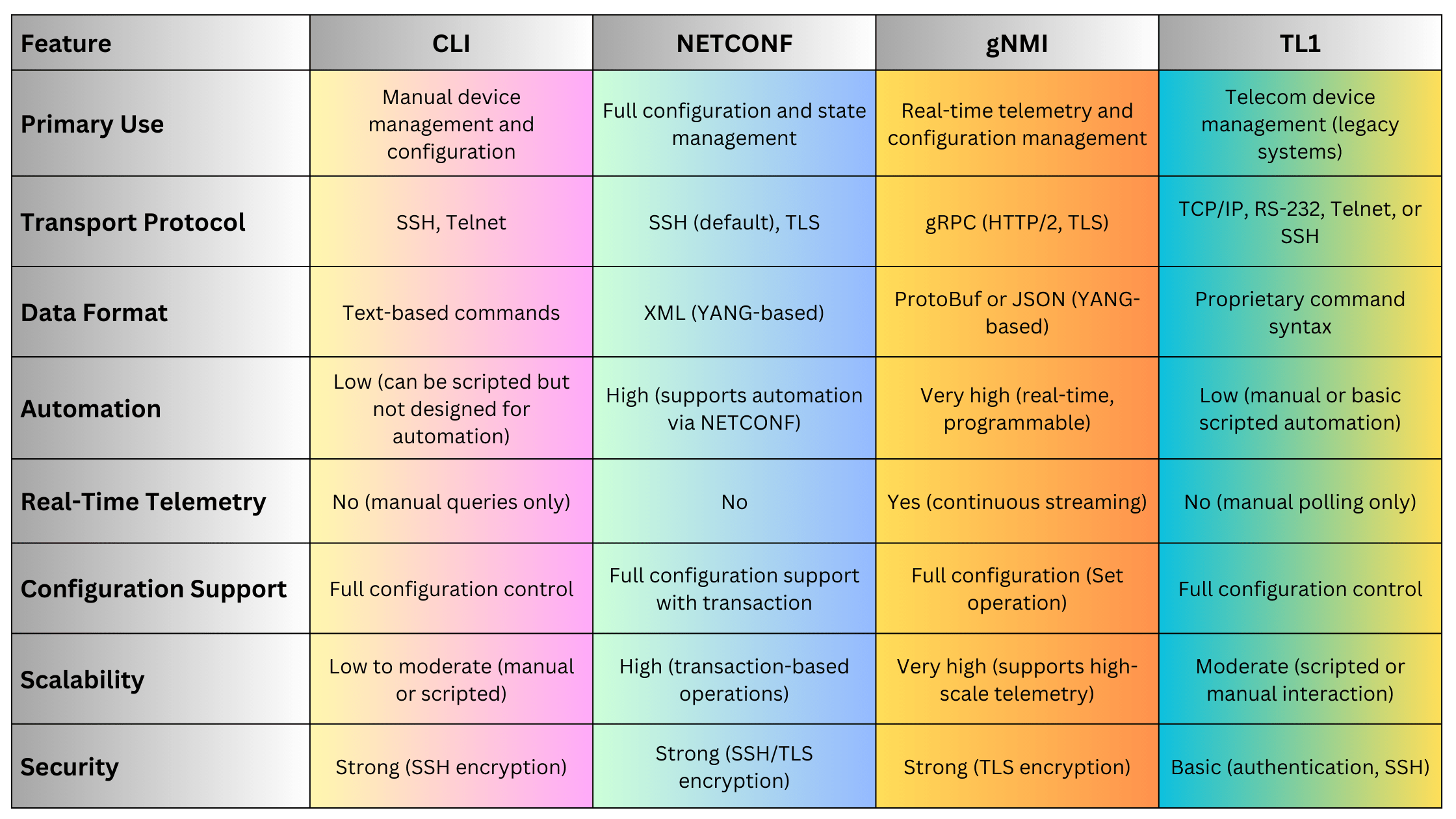
CLI examples for Networking and Optical Devices
Configuring an IP Address on a Router
To configure an IP address on a Cisco router, the following CLI commands can be used:
configure terminal
interface GigabitEthernet 0/1
ip address 192.168.1.1 255.255.255.0
no shutdown
This sequence configures GigabitEthernet 0/1 with an IP address of 192.168.1.1 and brings the interface online.
Monitoring Optical Power on a DWDM System
Network operators can use CLI to monitor the health of an optical transceiver on a DWDM system. The following command retrieves the power levels:
show interfaces optical-1/1/1 transceiverThis provides details on the receive and transmit power levels, temperature, and signal-to-noise ratio (SNR).
Setting an Optical Channel Power Level
To configure the power output of a specific optical channel on a DWDM system, the following CLI command can be used:
interface optical-1/1/1
transceiver power -2.0
This sets the output power to -2.0 dBm for optical interface 1/1/1.
Viewing Routing Information on a Router
To view the current routing table on a Cisco router, use the following command:
show ip routeThis displays the routing table, which shows the available routes, next-hop addresses, and metrics.
CLI Automation with Python Example
Although CLI is primarily a manual interface, it can be automated using scripting languages like Python. Here’s a simple Python script that uses Paramiko to connect to 1a Cisco device via SSH and retrieve interface status:
import paramiko

# Establish SSH connection
ssh = paramiko.SSHClient()
ssh.set_missing_host_key_policy(paramiko.AutoAddPolicy())
ssh.connect('192.168.1.1', username='admin', password='password')

# Execute CLI command
stdin, stdout, stderr = ssh.exec_command('show ip interface brief')
output = stdout.read().decode()

# Print the output
print(output)

# Close the connection
ssh.close()
This script connects to a Cisco device, runs the show ip interface brief command, and prints the output.
Summary
CLI (Command Line Interface) is a powerful and ubiquitous tool for managing network and optical devices. Its simplicity, direct access, and flexibility make it the preferred choice for many network engineers, especially in environments where manual configuration and troubleshooting are common. However, as networks grow in scale and complexity, modern protocols like NETCONF, gNMI, and OpenConfig offer more advanced features, including real-time telemetry, automation, and programmability. Despite these advancements, CLI remains a vital part of the network engineer’s toolkit, especially for legacy systems and smaller-scale operations.
")
TL1 (Transaction Language 1) is a command-line language used in telecommunication networks, particularly in managing optical networks. Developed in the 1980s, TL1 is one of the oldest network management protocols and remains a key protocol in legacy telecom systems. It is primarily used for managing telecommunication equipment like DWDM systems, SONET/SDH, and OTN devices, providing operators with the ability to configure, monitor, and control network elements via manual or automated commands.Lets explore the fundamentals of TL1, its command structure, how it is used in optical networks, advantages and disadvantages, and how it compares to modern network management protocols like NETCONF and gNMI. We will also provide examples of how TL1 can be used for managing optical devices.
What Is TL1?
TL1 (Transaction Language 1) is a standardized command-line interface designed to manage and control telecommunication network elements, especially those related to optical transport networks (OTNs), DWDM, SONET/SDH, and other carrier-grade telecommunication systems. Unlike modern protocols that are API-driven, TL1 is text-based and uses structured commands for device interaction, making it akin to traditional CLI (Command Line Interface).
Key Features:
- Command-based: TL1 relies on a simple command-response model, where commands are entered manually or sent via scripts.
- Human-readable: Commands and responses are structured as text, making it easy for operators to interpret.
- Wide Adoption in Optical Networks: TL1 is still prevalent in older optical network equipment, including systems from vendors like Alcatel-Lucent, Nokia, Huawei, and Fujitsu.
TL1 commands can be used to:
- Configure network elements (NEs), such as adding or removing circuits.
- Retrieve the status of NEs, such as the power levels of optical channels.
- Issue control commands, such as activating or deactivating ports.
TL1 Command Structure
The TL1 protocol is built around a structured command-response model, where each command has a specific format and triggers a predefined action on the network element.
Basic TL1 Command Syntax:
A standard TL1 command typically includes several parts:
<Verb>:[TID]:<AID>:<CTAG>::<Parameters>;- Verb: Specifies the action to be performed, such as SET, RTRV, ACT, DLT.
- TID (Target Identifier): Identifies the network element to which the command is being sent.
- AID (Access Identifier): Specifies the element or resource (e.g., port, channel) within the NE.
- CTAG (Correlation Tag): A unique identifier for the command, used to track the request and response.
- Parameters: Optional additional parameters for configuring the NE or specifying retrieval criteria.
Example of a TL1 Command:
Retrieve the status of an optical port:
RTRV-OPTPORT::OTN-1-3::ALL;In this example:
- RTRV-OPTPORT: The verb that requests the retrieval of optical port data.
- OTN-1-3: The AID specifying the OTN element and port number.
- ALL: Specifies that all relevant data for the optical port should be retrieved.
Common TL1 Commands for Optical Networks
TL1 commands are categorized by the type of action they perform, with the most common verbs being RTRV (retrieve), ACT (activate), SET (set parameters), and DLT (delete).
RTRV (Retrieve) Commands:
RTRV commands are used to gather status and performance information from optical devices. Examples include retrieving signal levels, operational states, and alarm statuses.
- Retrieve the optical power level on a specific port:
RTRV-OPTPORT::DWDM-1-2::ALL; - Retrieve alarm information for an optical channel:
RTRV-ALM-OPTCHAN::DWDM-1-3::ALL;
ACT (Activate) Commands:
ACT commands are used to enable or bring a resource (e.g., port, channel) into an operational state.
- Activate an optical channel:
ACT-OPTCHAN::DWDM-1-2-CH-5;
SET (Set Parameters) Commands:
SET commands allow operators to modify the configuration of network elements, such as setting power levels, modulation formats, or wavelengths for optical channels.
- Set the output power of a DWDM port:
SET-OPTPORT::DWDM-1-3::POWER=-3.5;
DLT (Delete) Commands:
DLT commands are used to remove or deactivate network elements, such as deleting a circuit or channel.
- Delete an optical channel:
DLT-OPTCHAN::DWDM-1-2-CH-5;
TL1 in Optical Networks
In optical networks, TL1 is commonly used for managing DWDM systems, OTN devices, and SONET/SDH equipment. Operators use TL1 to perform critical network operations, including:
Provisioning Optical Channels
TL1 commands allow operators to provision optical channels by setting parameters such as frequency, power, and modulation format. For example, setting up a new optical channel on a DWDM system:
ACT-OPTCHAN::DWDM-1-4-CH-7::FREQ=193.1GHz, POWER=-3.0dBm;This command provisions a new channel on DWDM port 1-4 at 193.1 GHz with a power output of -3 dBm.
Monitoring Optical Power Levels
Network operators can use TL1 to monitor the health of the optical network by retrieving real-time power levels from transponders and optical amplifiers:
RTRV-OPTPORT::DWDM-1-2::ALL;This command retrieves the power levels, signal-to-noise ratios (SNR), and other key metrics for the specified port.
Handling Alarms and Events
TL1 provides a way to monitor and handle alarms in optical networks. Operators can retrieve current alarms, acknowledge them, or clear them once the issue is resolved:
RTRV-ALM-OPTCHAN::DWDM-1-2::ALL;This command retrieves all active alarms on optical channel 1-2.
TL1 Advantages
Simplicity
TL1 is simple and easy to learn, especially for telecom engineers familiar with CLI-based management. The human-readable command structure allows for straightforward device management without the need for complex protocols.
Vendor Support
TL1 is widely supported by legacy optical networking devices from various vendors, including Ribbon, Cisco, Ciena, Alcatel-Lucent, Huawei, Nokia, and Fujitsu. This makes it a reliable tool for managing older telecom networks.
Customizability
Because TL1 is command-based, it can be easily scripted or automated using basic scripting languages. This makes it possible to automate repetitive tasks such as provisioning, monitoring, and troubleshooting in optical networks.
Granular Control
TL1 allows for granular control over individual network elements, making it ideal for configuring specific parameters, retrieving real-time status information, or responding to alarms.
TL1 Disadvantages
Limited Automation and Scalability
Compared to modern protocols like NETCONF and gNMI, TL1 lacks built-in automation capabilities. It is not well-suited for large-scale network automation or dynamic environments requiring real-time telemetry.
Proprietary Nature
While TL1 is standardized to an extent, each vendor often implements vendor-specific command sets or extensions. This means TL1 commands may vary slightly across devices from different vendors, leading to compatibility issues.
Lack of Real-Time Telemetry
TL1 is primarily designed for manual or scripted command entry. It lacks native support for real-time telemetry or continuous streaming of data, which is increasingly important in modern networks for performance monitoring and fault detection.
Obsolescence
As networks evolve towards software-defined networking (SDN) and automation, TL1 is gradually being phased out in favor of more modern protocols like NETCONF, RESTCONF, and gNMI, which offer better scalability, programmability, and real-time capabilities.
TL1 vs. Modern Protocols (NETCONF, gNMI, OpenConfig)
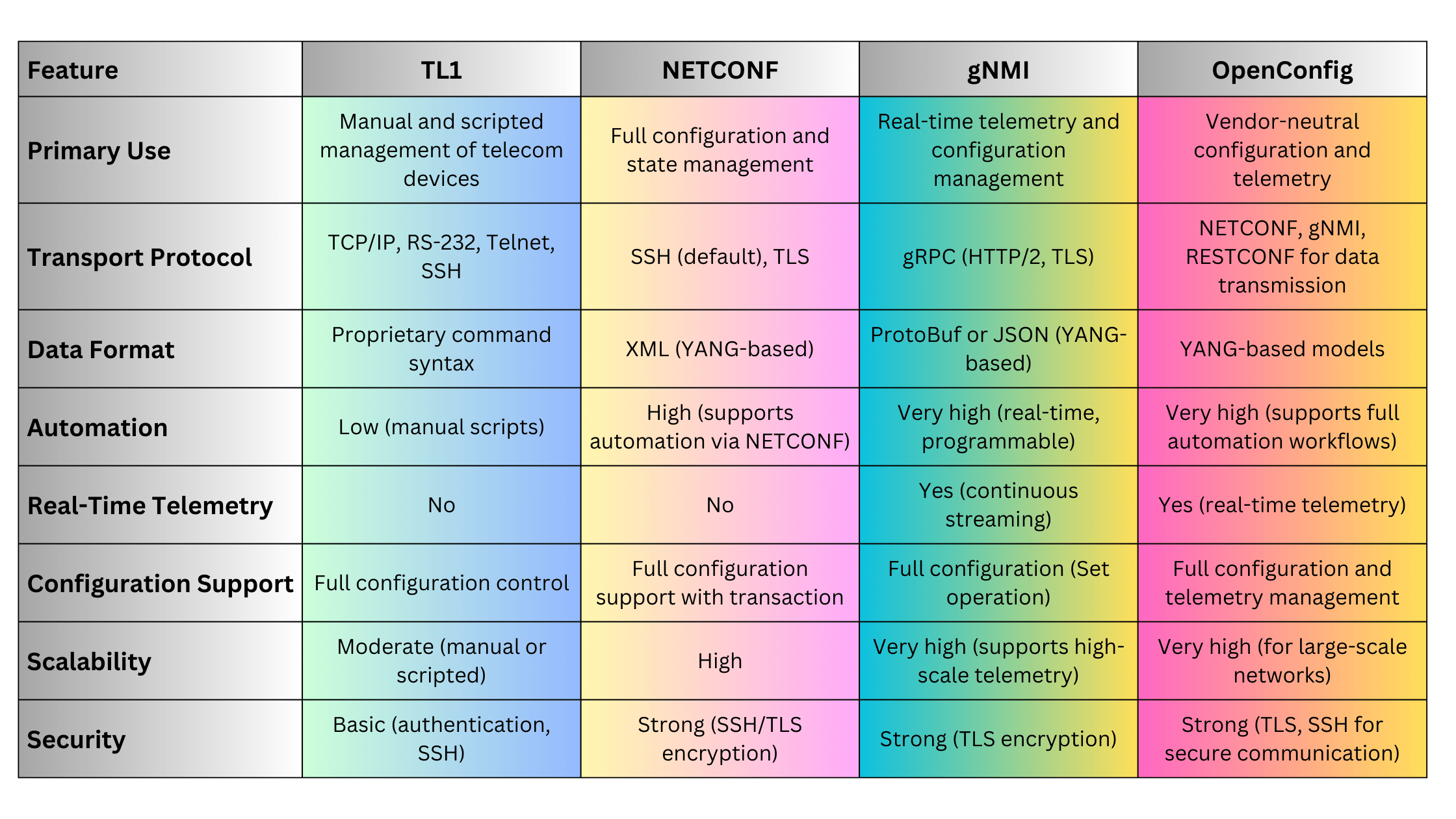
TL1 examples in Optical Networks
Provisioning an Optical Channel on a DWDM System
To provision an optical channel with specific parameters, such as frequency and power level, a TL1 command could look like this:
ACT-OPTCHAN::DWDM-1-2-CH-6::FREQ=193.3GHz, POWER=-2.5dBm;This command activates channel 6 on DWDM port 1-2 with a frequency of 193.3 GHz and an output power of -2.5 dBm.
Retrieving Optical Port Power Levels
Operators can retrieve the power levels for a specific optical port using the following command:
RTRV-OPTPORT::DWDM-1-3::ALL;This retrieves the current signal levels, power output, and other metrics for DWDM port 1-3.
Deactivating an Optical Channel
If an optical channel needs to be deactivated or removed, the following command can be used:
DLT-OPTCHAN::DWDM-1-2-CH-6;This deletes channel 6 on DWDM port 1-2, effectively taking it out of service.
Summary
TL1 remains a key protocol in the management of legacy optical networks, providing telecom operators with granular control over their network elements. Its command-based structure, simplicity, and vendor support have made it an enduring tool for managing DWDM, OTN, and SONET/SDH systems. However, with the advent of modern, programmable protocols like NETCONF, gNMI, and OpenConfig, TL1’s role is diminishing as networks evolve toward automation, real-time telemetry, and software-defined networking.
Reference
")
As modern networks scale, the demand for real-time monitoring and efficient management of network devices has grown significantly. Traditional methods of network monitoring, such as SNMP, often fall short when it comes to handling the dynamic and high-performance requirements of today’s networks. gNMI (gRPC Network Management Interface), combined with streaming telemetry, provides a more efficient, scalable, and programmable approach to managing and monitoring network devices.Lets explore gNMI, its architecture, key features, how it differs from traditional protocols like SNMP and NETCONF, and its advantages. We will also look at how streaming telemetry works with gNMI to deliver real-time data from network devices, including use cases in modern networking and optical networks.
What Is gNMI?
gNMI (gRPC Network Management Interface) is a network management protocol developed by Google and other major tech companies to provide real-time configuration and state retrieval from network devices. Unlike traditional polling methods, gNMI operates over gRPC (Google Remote Procedure Call) and supports streaming telemetry, which provides real-time updates on network performance and device health.
Key Features:
- Real-Time Telemetry: gNMI enables real-time, high-frequency data streaming from devices to a centralized monitoring system.
- gRPC-Based: It uses the high-performance gRPC framework for communication, which is built on HTTP/2 and supports bidirectional streaming, ensuring low latency and high throughput.
- Full Configuration Support: gNMI allows network operators to configure devices programmatically and retrieve both operational and configuration data.
- Data Model Driven: gNMI uses YANG models to define the data being monitored or configured, ensuring consistency across vendors.
gNMI and Streaming Telemetry Overview
Streaming telemetry allows network devices to push data continuously to a monitoring system without the need for constant polling by management tools. gNMI is the protocol that facilitates the delivery of this telemetry data using gRPC, which provides a reliable and efficient means of communication.
With gNMI, network operators can:
- Stream performance metrics, such as CPU usage, bandwidth utilization, and link health, at granular intervals.
- Set up real-time alerts for threshold breaches (e.g., high latency, packet loss).
- Push configuration updates to devices dynamically and validate changes in real-time.
gNMI Architecture
gNMI operates in a client-server model, with the following components:
- gNMI Client: The application or system (often a monitoring tool or automation platform) that sends configuration requests or subscribes to telemetry streams from devices.
- gNMI Server: The network device (router, switch, optical device) that supports gNMI and responds to configuration requests or streams telemetry data.
- gRPC Transport: gNMI uses gRPC as its underlying transport layer. gRPC operates over HTTP/2, supporting bidirectional streaming and ensuring low-latency communication.
gNMI Operations
gNMI supports several operations for interacting with network devices:
- Get: Retrieves the current configuration or operational state of the device.
- Set: Pushes a new configuration or modifies an existing one.
- Subscribe: Subscribes to real-time telemetry updates from the device. This is the core of streaming telemetry in gNMI.
- On-Change: Data is pushed only when there is a change in the monitored metric (e.g., interface goes up/down).
- Sampled: Data is pushed at regular intervals, regardless of changes.
- Capabilities: Queries the device to determine the supported YANG models and features.
How gNMI Works: Streaming Telemetry Example
In traditional SNMP-based monitoring, devices are polled periodically, and data is retrieved based on requests from the monitoring system. This method introduces latency and can miss important real-time events. Streaming telemetry, on the other hand, allows network devices to continuously push real-time data to the monitoring system, providing better visibility into network performance.
Streaming Telemetry with gNMI:
- Subscribe to Metrics: The gNMI client (e.g., a telemetry collector) subscribes to specific metrics from the device, such as interface statistics or CPU usage.
- Data Streaming: The gNMI server on the device streams updates to the client either on-change or at specified intervals.
- Data Collection: The telemetry collector processes the streamed data and provides real-time insights, dashboards, or alerts based on predefined thresholds.
Example of a gNMI Subscription to Monitor Optical Channel Power Levels:
gnmi_subscribe -target_addr "192.168.1.10:57400" -tls -username admin -password admin \ -path "/optical-channel/state/output-power" -mode "sample" -interval "10s"In this example, the gNMI client subscribes to the output power of an optical channel, receiving updates every 10 seconds.
gNMI vs. Traditional Protocols (SNMP, NETCONF)
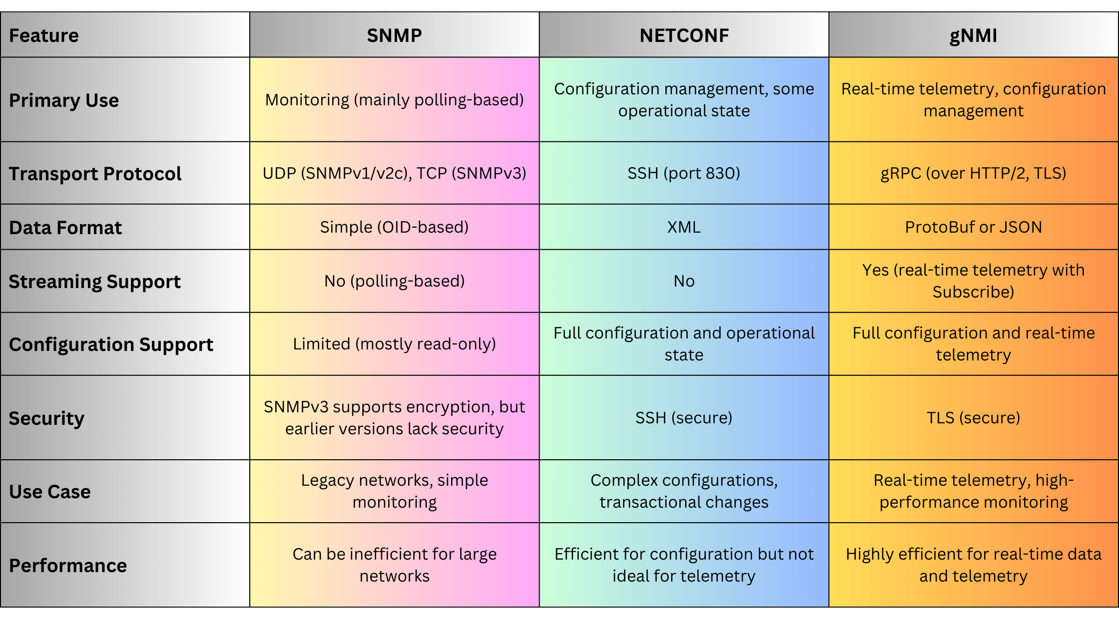
gNMI Use Cases
Real-Time Network Monitoring
gNMI is ideal for real-time monitoring in dynamic networks where performance metrics need to be collected continuously. With on-change and sampled telemetry, operators can monitor:
- Interface statistics: Monitor packet drops, errors, and link status changes.
- CPU/Memory usage: Track the health of devices and identify potential bottlenecks.
- Optical signal metrics: For optical networks, monitor key metrics like signal power, bit error rate (BER), and latency in real-time.
Automated Network Configuration
gNMI’s Set operation allows network operators to push configurations programmatically. For example, operators can automate the deployment of configurations across thousands of devices, ensuring consistency and reducing manual effort.
Streaming Telemetry in Optical Networks
In optical networks, gNMI plays a crucial role in monitoring and managing optical channels and transponders. For example, gNMI can be used to:
- Stream telemetry data on optical power levels, wavelength performance, and optical amplifiers.
- Dynamically configure optical channel parameters, such as frequency and power output, and monitor changes in real time.
Example: Streaming Telemetry from an Optical Device:
gnmi_subscribe -target_addr "10.0.0.5:57400" -tls -username admin -password admin \ -path "/optical-channel/state/frequency" -mode "on_change"This command subscribes to the optical channel’s frequency and receives real-time updates whenever the frequency changes.
Advantages of gNMI and Streaming Telemetry
gNMI, combined with streaming telemetry, offers numerous advantages:
- Real-Time Data: Provides immediate access to changes in network performance, allowing operators to react faster to network issues.
- Efficiency: Instead of polling devices for status, telemetry streams data as it becomes available, reducing network overhead and improving performance in large-scale networks.
- High Throughput: gRPC’s low-latency, bidirectional streaming makes gNMI ideal for handling the high-frequency data updates required in modern networks.
- Vendor Agnostic: gNMI leverages standardized YANG models, making it applicable across multi-vendor environments.
- Secure Communication: gNMI uses TLS to secure data streams, ensuring that telemetry data and configuration changes are encrypted.
Disadvantages of gNMI
While gNMI provides significant improvements over traditional protocols, there are some challenges:
- Complexity: Implementing gNMI and streaming telemetry requires familiarity with YANG models, gRPC, and modern networking concepts.
- Infrastructure Requirements: Streaming telemetry generates large volumes of data, requiring scalable telemetry collectors and back-end systems capable of processing and analyzing the data in real-time.
- Limited Legacy Support: Older devices may not support gNMI, meaning that hybrid environments may need to use SNMP or NETCONF alongside gNMI.
gNMI and Streaming Telemetry Example for Optical Networks
Imagine a scenario in an optical transport network (OTN) where it is crucial to monitor the power levels of optical channels in real-time to ensure the stability of long-haul links.
Step 1: Set Up a gNMI Subscription
Network operators can set up a gNMI subscription to monitor the optical power of channels at regular intervals, ensuring that any deviation from expected power levels is immediately reported.
gnmi_subscribe -target_addr "10.0.0.8:57400" -tls -username admin -password admin \ -path "/optical-channel/state/output-power" -mode "sample" -interval "5s"Step 2: Real-Time Data Streaming
The telemetry data from the optical transponder is streamed every 5 seconds, allowing operators to track power fluctuations and quickly detect any potential signal degradation.
Step 3: Trigger Automated Actions
If the power level crosses a predefined threshold, automated actions (e.g., notifications or adjustments) can be triggered.
gNMI vs. Other Telemetry Approaches: A Quick Comparison
Summary
gNMI and streaming telemetry are essential tools for modern network management, particularly in dynamic environments requiring real-time visibility into network performance. By replacing traditional polling-based methods with real-time data streams, gNMI provides a more efficient, scalable, and secure approach to monitoring and configuring devices. The protocol’s integration with YANG data models ensures vendor neutrality and standardization, while its use of gRPC enables high-performance, low-latency communication. As networks evolve, particularly in areas like optical networking, gNMI and streaming telemetry will continue to play a pivotal role in ensuring operational efficiency and network reliability.
")
OpenConfig is an open-source, vendor-neutral initiative designed to address the growing complexity of managing modern network infrastructures. It provides standardized models for configuring and monitoring network devices, focusing on programmability and automation. OpenConfig was created by large-scale network operators to address the limitations of traditional, vendor-specific configurations, allowing operators to manage devices from different vendors using a unified data model and interfaces.Lets explore OpenConfig, its architecture, key use cases, comparison with other network configuration approaches, and its advantages and disadvantages.
What is OpenConfig?
OpenConfig is a set of open-source, vendor-agnostic YANG models that standardize network configuration and operational state management across different devices and vendors. It focuses on enabling programmable networks, offering network operators the ability to automate, manage, and monitor their networks efficiently.
OpenConfig allows network administrators to:
- Use the same data models for configuration and monitoring across multi-vendor environments.
- Enable network programmability and automation with tools like NETCONF, gNMI, and RESTCONF.
- Standardize network management by abstracting the underlying hardware and software differences between vendors.
OpenConfig and YANG
At the heart of OpenConfig is YANG (Yet Another Next Generation), a data modeling language used to define the structure of configuration and operational data. YANG models describe the structure, types, and relationships of network elements in a hierarchical way, providing a common language for network devices.
Key Features of OpenConfig YANG Models:
- Vendor-neutral: OpenConfig models are designed to work across devices from different vendors, enabling interoperability and reducing complexity.
- Modular: OpenConfig models are modular, which allows for easy extension and customization for specific network elements (e.g., BGP, interfaces, telemetry).
- Versioned: The models are versioned, enabling backward compatibility and smooth upgrades.
Example of OpenConfig YANG Model for Interfaces:
module openconfig-interfaces {
  namespace "http://openconfig.net/yang/interfaces";
  prefix "oc-if";

  container interfaces {
    list interface {
      key "name";
      leaf name {
        type string;
      }
      container config {
        leaf description {
          type string;
        }
        leaf enabled {
          type boolean;
        }
      }
    }
  }
}
This model defines the structure for configuring network interfaces using OpenConfig. It includes configuration elements like name, description, and enabled status.
How OpenConfig Works
OpenConfig models are typically used in conjunction with network management protocols like NETCONF, gNMI, or RESTCONF to configure and monitor devices. These protocols interact with OpenConfig YANG models to retrieve or update configurations programmatically.
Here’s how OpenConfig works with these protocols:
- NETCONF: Communicates with devices to send or retrieve configuration and operational data in a structured XML format, using OpenConfig YANG models.
- gNMI (gRPC Network Management Interface): A more modern approach, gNMI uses a gRPC-based transport mechanism to send and receive configuration data in real-time using OpenConfig YANG models. It is designed for more efficient streaming telemetry.
- RESTCONF: Provides a RESTful interface over HTTP/HTTPS for managing configurations using OpenConfig models.
OpenConfig in Optical Networks
OpenConfig is particularly valuable in optical networks, where multiple vendors provide devices like DWDM systems, optical transponders, and OTN equipment. Managing these devices can be complex due to vendor-specific configurations and proprietary management interfaces. OpenConfig simplifies optical network management by providing standardized models for:
- Optical Channel Management: Define configurations for optical transponders and manage channel characteristics such as wavelength, power, and modulation.
- DWDM Network Elements: Configure and monitor Dense Wavelength Division Multiplexing systems in a vendor-neutral way.
- Optical Amplifiers: Manage and monitor amplifiers in long-haul networks using standardized OpenConfig models.
Example: OpenConfig YANG Model for Optical Channels
OpenConfig provides models like openconfig-optical-transport-line-common for optical networks. Here’s an example snippet of configuring an optical channel:
module openconfig-optical-transport-line-common {
  container optical-channel {
    list channel {
      key "name";
      leaf name {
        type string;
      }
      container config {
        leaf frequency {
          type uint32;
        }
        leaf target-output-power {
          type decimal64;
        }
      }
    }
  }
}
This YANG model defines the structure for configuring an optical channel, allowing operators to set parameters like frequency and target-output-power.
Key Components of OpenConfig
OpenConfig has several key components that make it effective for managing network devices:
Standardized Models
OpenConfig models cover a wide range of network elements and functions, from BGP and VLANs to optical transport channels. These models are designed to work with any device that supports OpenConfig, regardless of the vendor.
Streaming Telemetry
OpenConfig supports streaming telemetry, which allows real-time monitoring of network state and performance using protocols like gNMI. This approach provides a more efficient alternative to traditional polling methods like SNMP.
Declarative Configuration
OpenConfig uses declarative configuration methods, where the desired end-state of the network is defined and the system automatically adjusts to achieve that state. This contrasts with traditional imperative methods, where each step of the configuration must be manually specified.
OpenConfig Protocols: NETCONF vs. gNMI vs. RESTCONF
While OpenConfig provides the data models, various protocols are used to interact with these models. The table below provides a comparison of these protocols:
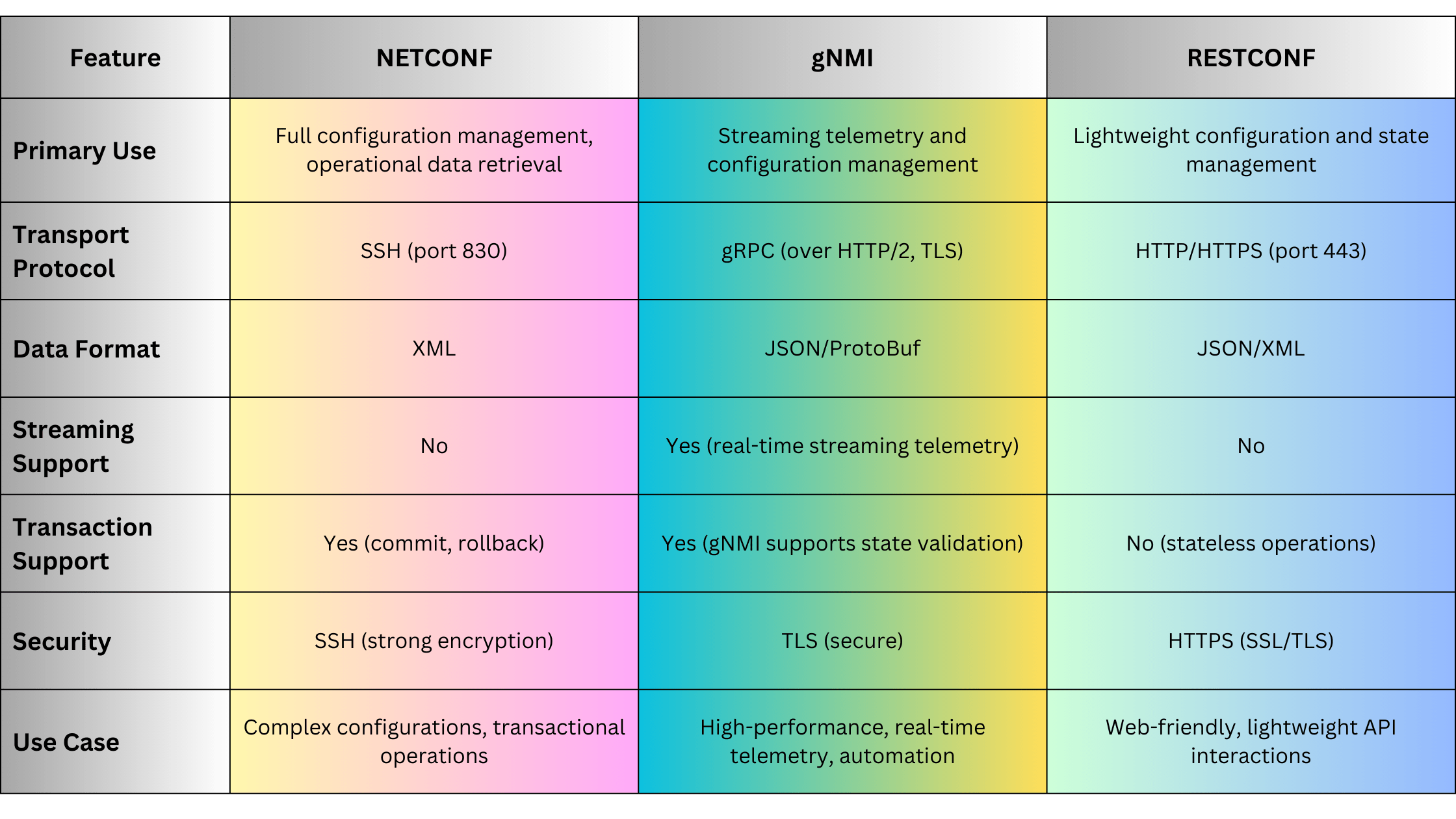
When to Use OpenConfig
OpenConfig is particularly useful in several scenarios:
Multi-Vendor Networks
OpenConfig is ideal for networks that use devices from multiple vendors, as it standardizes configurations and monitoring across all devices, reducing the need for vendor-specific tools.
Large-Scale Automation
For networks requiring high levels of automation, OpenConfig enables the use of programmatic configuration and monitoring. Combined with gNMI, it provides real-time streaming telemetry for dynamic network environments.
Optical Networks
OpenConfig’s models for optical networks allow network operators to manage complex optical channels, amplifiers, and transponders in a standardized way, simplifying the management of DWDM systems and OTN devices.
Advantages of OpenConfig
OpenConfig provides several advantages for network management:
- Vendor Neutrality: OpenConfig removes the complexity of vendor-specific configurations, providing a unified way to manage multi-vendor environments.
- Programmability: OpenConfig models are ideal for automation and programmability, especially when integrated with tools like NETCONF, gNMI, or RESTCONF.
- Streaming Telemetry: OpenConfig’s support for streaming telemetry enables real-time monitoring of network state and performance, improving visibility and reducing latency for performance issues.
- Extensibility: OpenConfig YANG models are modular and extensible, allowing for customization and adaptation to new use cases and technologies.
- Declarative Configuration: Allows network operators to define the desired state of the network, reducing the complexity of manual configurations and ensuring consistent network behavior.
Disadvantages of OpenConfig
Despite its benefits, OpenConfig has some limitations:
- Complexity: OpenConfig YANG models can be complex to understand and implement, particularly for network operators who are not familiar with data modeling languages like YANG.
- Learning Curve: Network administrators may require additional training to fully leverage OpenConfig and associated technologies like NETCONF, gNMI, and YANG.
- Limited Legacy Support: Older devices may not support OpenConfig, meaning that legacy networks may require hybrid management strategies using traditional tools alongside OpenConfig.
OpenConfig in Action: Example for Optical Networks
Imagine a scenario where you need to configure an optical transponder using OpenConfig to set the frequency and target power of an optical channel. Here’s an example using OpenConfig with gNMI:
Step 1: Configure Optical Channel Parameters
{
  "openconfig-optical-transport-line-common:optical-channel": {
    "channel": {
      "name": "channel-1",
      "config": {
        "frequency": 193400,
        "target-output-power": -3.5
      }
    }
  }
}
Step 2: gNMI Configuration
Send the configuration using a gNMI client:
gnmi_set -target_addr "192.168.1.10:57400" -tls -username admin -password admin -update_path "/optical-channel/channel[name=channel-1]/config/frequency" -update_value 193400This command sends the target frequency value of 193.4 THz to the optical transponder using gNMI.
OpenConfig vs. Traditional Models: A Quick Comparison
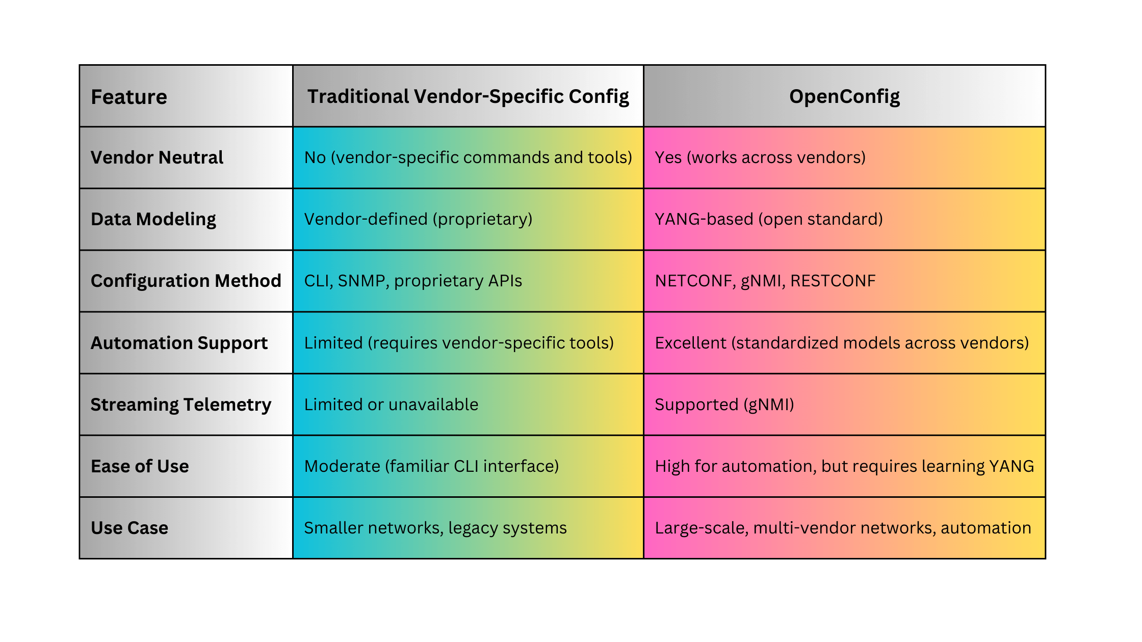
Summary
OpenConfig has revolutionized network device management by providing a standardized, vendor-neutral framework for configuration and monitoring. Its YANG-based models allow for seamless multi-vendor network management, while protocols like NETCONF and gNMI provide the programmability and real-time telemetry needed for modern, automated networks. Although it comes with a learning curve and complexity, the benefits of standardization, scalability, and automation make OpenConfig an essential tool for managing large-scale networks, particularly in environments that include both traditional and optical devices.
Reference
")
Syslog is one of the most widely used protocols for logging system events, providing network and optical device administrators with the ability to collect, monitor, and analyze logs from a wide range of devices. This protocol is essential for network monitoring, troubleshooting, security audits, and regulatory compliance. Originally developed in the 1980s, Syslog has since become a standard logging protocol, used in various network and telecommunications environments, including optical devices.Lets explore Syslog, its architecture, how it works, its variants, and use cases. We will also look at its implementation on optical devices and how to configure and use it effectively to ensure robust logging in network environments.
What Is Syslog?
Syslog (System Logging Protocol) is a protocol used to send event messages from devices to a central server called a Syslog server. These event messages are used for various purposes, including:
- Monitoring: Identifying network performance issues, equipment failures, and status updates.
- Security: Detecting potential security incidents and compliance auditing.
- Troubleshooting: Diagnosing issues in real-time or after an event.
Syslog operates over UDP (port 514) by default, but can also use TCP to ensure reliability, especially in environments where message loss is unacceptable. Many network devices, including routers, switches, firewalls, and optical devices such as optical transport networks (OTNs) and DWDM systems, use Syslog to send logs to a central server.
How Syslog Works
Syslog follows a simple architecture consisting of three key components:
- Syslog Client: The network device (such as a switch, router, or optical transponder) that generates log messages.
- Syslog Server: The central server where log messages are sent and stored. This could be a dedicated logging solution like Graylog, RSYSLOG, Syslog-ng, or a SIEM system.
- Syslog Message: The log data itself, consisting of several fields such as timestamp, facility, severity, hostname, and message content.
Syslog Message Format
Syslog messages contain the following fields:
- Priority (PRI): A combination of facility and severity, indicating the type and urgency of the message.
- Timestamp: The time at which the event occurred.
- Hostname/IP: The device generating the log.
- Message: A human-readable description of the event.
Example of a Syslog Message:
<34>Oct 10 13:22:01 router-1 interface GigabitEthernet0/1 downThis message shows that the device with hostname router-1 logged an event at Oct 10 13:22:01, indicating that the GigabitEthernet0/1 interface went down.
Syslog Severity Levels
Syslog messages are categorized by severity to indicate the importance of each event. Severity levels range from 0 (most critical) to 7 (informational):
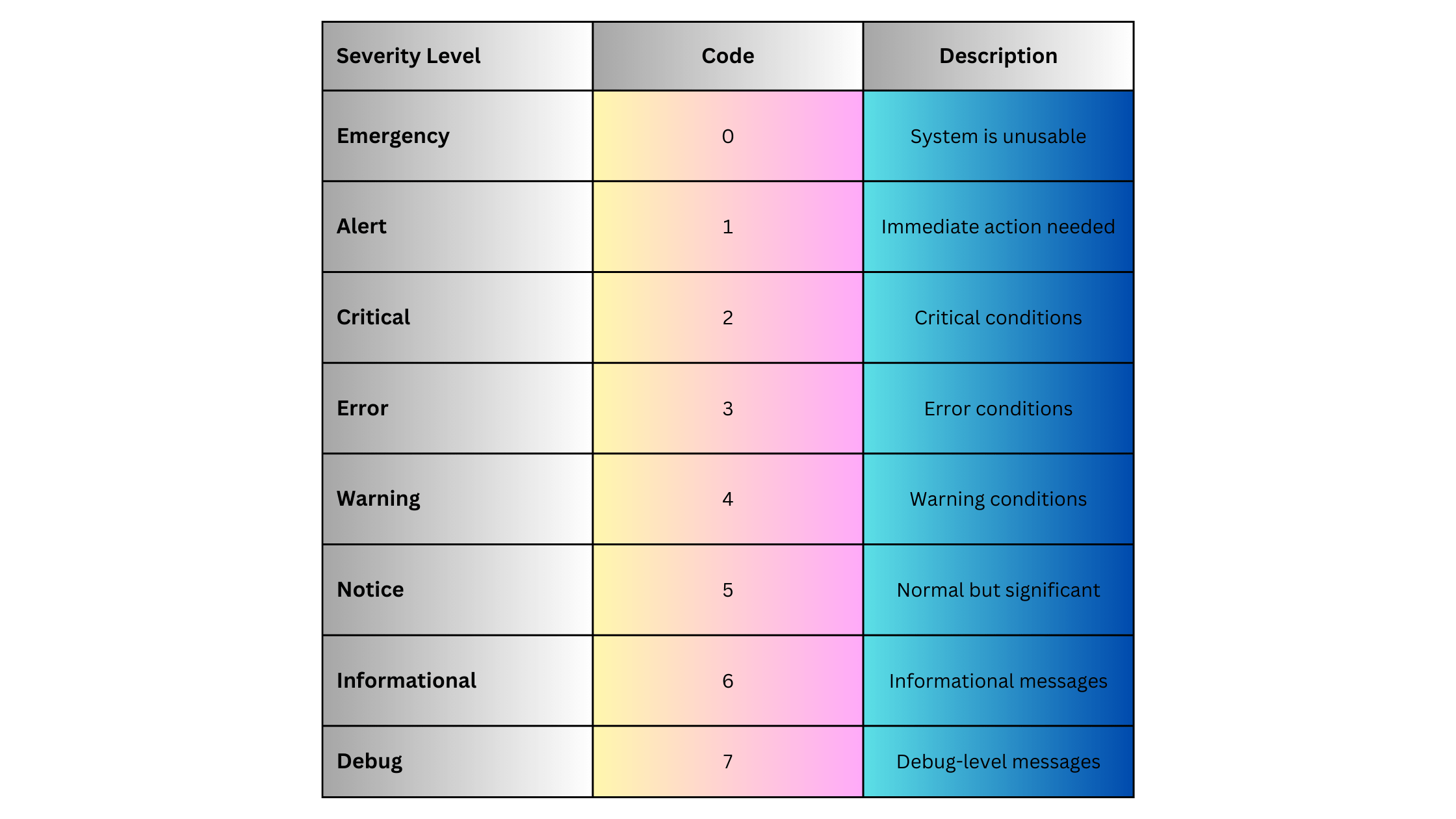
Syslog Facilities
Syslog messages also include a facility code that categorizes the source of the log message. Commonly used facilities include:

Each facility is paired with a severity level to determine the Priority (PRI) of the Syslog message.
Syslog in Optical Networks
Syslog is crucial in optical networks, particularly in managing and monitoring optical transport devices, DWDM systems, and Optical Transport Networks (OTNs). These devices generate various logs related to performance, alarms, and system health, which can be critical for maintaining service-level agreements (SLAs) in telecom environments.
Common Syslog Use Cases in Optical Networks:
- DWDM System Monitoring:
- Track optical signal power levels, bit error rates, and link status in real-time.
- Example: “DWDM Line 1 signal degraded, power level below threshold.”
- OTN Alarms:
- Log alarms related to client signal loss, multiplexing issues, and channel degradations.
- Example: “OTN client signal failure on port 3.”
- Performance Monitoring:
- Monitor latency, jitter, and packet loss in the optical transport network, essential for high-performance links.
- Example: “Performance threshold breach on optical channel, jitter exceeded.”
- Hardware Failure Alerts:
- Receive notifications for hardware-related failures, such as power supply issues or fan failures.
- Example: “Power supply failure on optical amplifier module.”
These logs can be critical for network operations centers (NOCs) to detect and resolve problems in the optical network before they impact service.
Syslog Example for Optical Devices
Here’s an example of a Syslog message from an optical device, such as a DWDM system:
<22>Oct 12 10:45:33 DWDM-1 optical-channel-1 signal degradation, power level -5.5dBm, threshold -5dBmThis message shows that on DWDM-1, optical-channel-1 is experiencing signal degradation, with the power level reported at -5.5dBm, below the threshold of -5dBm. Such logs are crucial for maintaining the integrity of the optical link.
Syslog Variants and Extensions
Several extensions and variants of Syslog add advanced functionality:
Reliable Delivery (RFC 5424)
The traditional UDP-based Syslog delivery method can lead to log message loss. To address this, Syslog has been extended to support TCP-based delivery and even Syslog over TLS (RFC 5425), which ensures encrypted and reliable message delivery, particularly useful for secure environments like data centers and optical networks.
Structured Syslog
To standardize log formats across different vendors and devices, Structured Syslog (RFC 5424) allows logs to include structured data in a key-value format, enabling easier parsing and analysis.
Syslog Implementations for Network and Optical Devices
To implement Syslog in network or optical environments, the following steps are typically involved:
Step 1: Enable Syslog on Devices
For optical devices such as Cisco NCS (Network Convergence System) or Huawei OptiX OSN, Syslog can be enabled to forward logs to a central Syslog server.
Example for Cisco Optical Device:
logging host 192.168.1.10
logging trap warnings
In this example:
-
- logging host configures the Syslog server’s IP.
- logging trap warnings ensures that only messages with a severity of warning (level 4) or higher are forwarded.
Step 2: Configure Syslog Server
Install a Syslog server (e.g., Syslog-ng, RSYSLOG, Graylog). Configure the server to receive and store logs from optical devices.
Example for RSYSLOG:
module(load="imudp")
input(type="imudp" port="514")
*.* /var/log/syslog
Step 3: Configure Log Rotation and Retention
Set up log rotation to manage disk space on the Syslog server. This ensures older logs are archived and only recent logs are stored for immediate access.
Syslog Advantages
Syslog offers several advantages for logging and network management:
- Simplicity: Syslog is easy to configure and use on most network and optical devices.
- Centralized Management: It allows for centralized log collection and analysis, simplifying network monitoring and troubleshooting.
- Wide Support: Syslog is supported across a wide range of devices, including network switches, routers, firewalls, and optical systems.
- Real-time Alerts: Syslog can provide real-time alerts for critical issues like hardware failures or signal degradation.
Syslog Disadvantages
Syslog also has some limitations:
- Lack of Reliability (UDP): If using UDP, Syslog messages can be lost during network congestion or failures. This can be mitigated by using TCP or Syslog over TLS.
- Unstructured Logs: Syslog messages can vary widely in format, which can make parsing and analyzing logs more difficult. However, structured Syslog (RFC 5424) addresses this issue.
- Scalability: In large networks with hundreds or thousands of devices, Syslog servers can become overwhelmed with log data. Solutions like log aggregation or log rotation can help manage this.
Syslog Use Cases
Syslog is widely used in various scenarios:
Network Device Monitoring
-
- Collect logs from routers, switches, and firewalls for real-time network monitoring.
- Detect issues such as link flaps, protocol errors, and device overloads.
Optical Transport Networks (OTN) Monitoring
-
- Track optical signal health, link integrity, and performance thresholds in DWDM systems.
- Generate alerts when signal degradation or failures occur on critical optical links.
Security Auditing
-
- Log security events such as unauthorized login attempts or firewall rule changes.
- Centralize logs for compliance with regulations like GDPR, HIPAA, or PCI-DSS.
Syslog vs. Other Logging Protocols: A Quick Comparison
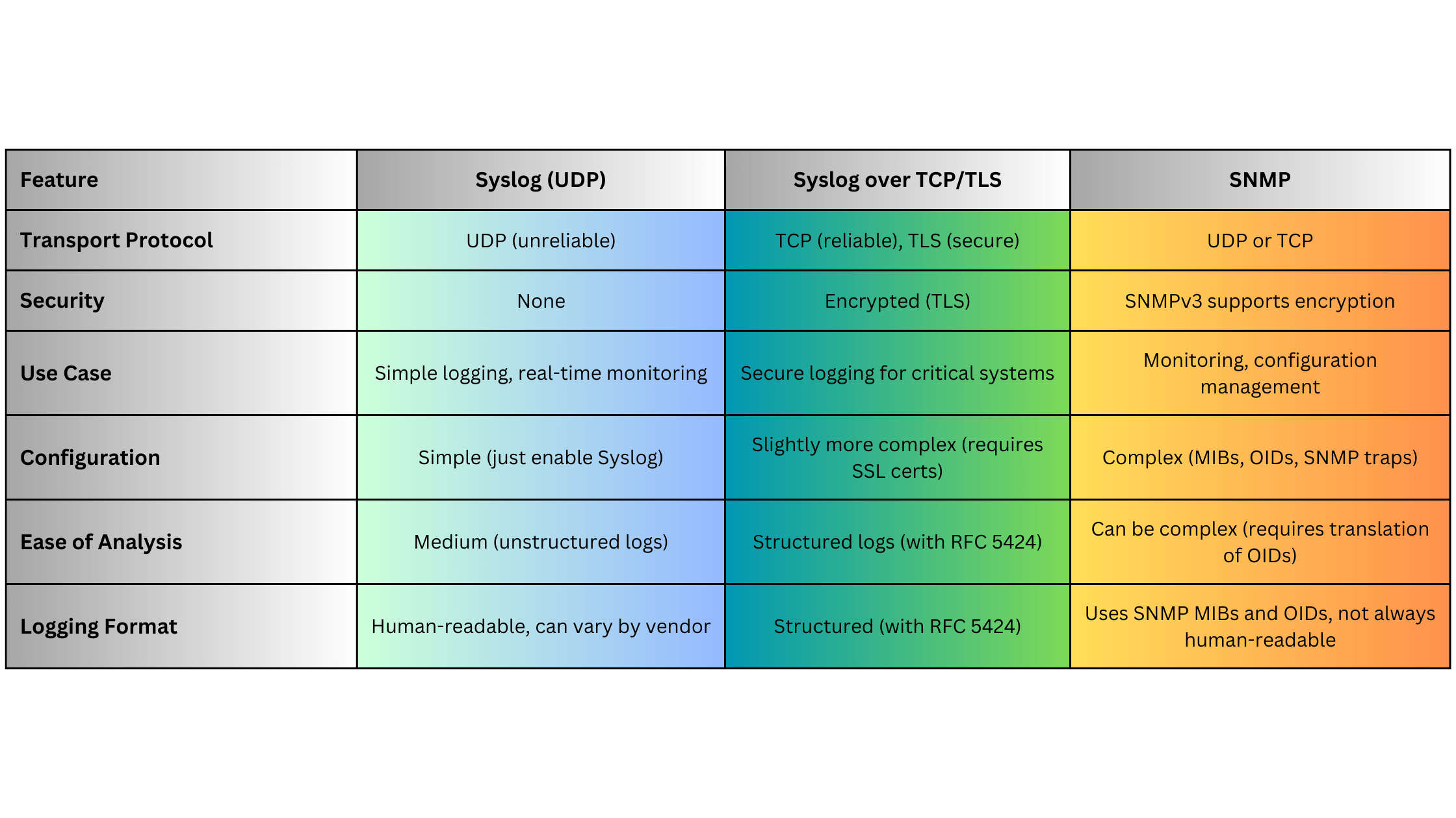
Syslog Use Case for Optical Networks
Imagine a scenario where an optical transport network (OTN) link begins to degrade due to a fiber issue:
- The OTN transponder detects a degradation in signal power.
- The device generates a Syslog message indicating the power level is below a threshold.
- The Syslog message is sent to a Syslog server for real-time alerting.
- The network administrator is notified immediately, allowing them to dispatch a technician to inspect the fiber and prevent downtime.
Example Syslog Message:
<27>Oct 13 14:10:45 OTN-Transponder-1 optical-link-3 signal degraded, power level -4.8dBm, threshold -4dBmSummary
Syslog remains one of the most widely-used protocols for logging and monitoring network and optical devices due to its simplicity, versatility, and wide adoption across vendors. Whether managing a large-scale DWDM system, monitoring OTNs, or tracking network security, Syslog provides an essential mechanism for real-time logging and event monitoring. Its limitations, such as unreliable delivery via UDP, can be mitigated by using Syslog over TCP or TLS in secure or mission-critical environments.
")
RESTCONF (RESTful Configuration Protocol) is a network management protocol designed to provide a simplified, REST-based interface for managing network devices using HTTP methods. RESTCONF builds on the capabilities of NETCONF by making network device configuration and operational data accessible over the ubiquitous HTTP/HTTPS protocol, allowing for easy integration with web-based tools and services. It leverages the YANG data modeling language to represent configuration and operational data, providing a modern, API-driven approach to managing network infrastructure. Lets explore the fundamentals of RESTCONF, its architecture, how it compares with NETCONF, the use cases it serves, and the benefits and drawbacks of adopting it in your network.
What Is RESTCONF?
RESTCONF (Representational State Transfer Configuration) is defined in RFC 8040 and provides a RESTful API that enables network operators to access, configure, and manage network devices using HTTP methods such as GET, POST, PUT, PATCH, and DELETE. Unlike NETCONF, which uses a more complex XML-based communication, RESTCONF adopts a simple REST architecture, making it easier to work with in web-based environments and for integration with modern network automation tools.
Key Features:
- HTTP-based: RESTCONF is built on the widely-adopted HTTP/HTTPS protocols, making it compatible with web services and modern applications.
- Data Model Driven: Similar to NETCONF, RESTCONF uses YANG data models to define how configuration and operational data are structured.
- JSON/XML Support: RESTCONF allows the exchange of data in both JSON and XML formats, giving it flexibility in how data is represented and consumed.
- Resource-Based: RESTCONF treats network device configurations and operational data as resources, allowing them to be easily manipulated using HTTP methods.
How RESTCONF Works
RESTCONF operates as a client-server model, where the RESTCONF client (typically a web application or automation tool) communicates with a RESTCONF server (a network device) using HTTP. The protocol leverages HTTP methods to interact with the data represented by YANG models.
HTTP Methods in RESTCONF:
- GET: Retrieve configuration or operational data from the device.
- POST: Create new configuration data on the device.
- PUT: Update existing configuration data.
- PATCH: Modify part of the existing configuration.
- DELETE: Remove configuration data from the device.
RESTCONF provides access to various network data through a well-defined URI structure, where each part of the network’s configuration or operational data is treated as a unique resource. This resource-centric model allows for easy manipulation and retrieval of network data.
RESTCONF URI Structure and Example
RESTCONF URIs provide access to different parts of a device’s configuration or operational data. The general structure of a RESTCONF URI is as follows:
/restconf/<resource-type>/<data-store>/<module>/<container>/<leaf>
- resource-type: Defines whether you are accessing data (
/data) or operations (/operations). - data-store: The datastore being accessed (e.g.,
/runningor/candidate). - module: The YANG module that defines the data you are accessing.
- container: The container (group of related data) within the module.
- leaf: The specific data element being retrieved or modified.
Example: If you want to retrieve the current configuration of interfaces on a network device, the RESTCONF URI might look like this:
GET /restconf/data/ietf-interfaces:interfacesThis request retrieves all the interfaces on the device, as defined in the ietf-interfaces YANG model.
RESTCONF Data Formats
RESTCONF supports two primary data formats for representing configuration and operational data:
- JSON (JavaScript Object Notation): A lightweight, human-readable data format that is widely used in web applications and REST APIs.
- XML (Extensible Markup Language): A more verbose, structured data format commonly used in network management systems.
Most modern implementations prefer JSON due to its simplicity and efficiency, particularly in web-based environments.
RESTCONF and YANG
Like NETCONF, RESTCONF relies on YANG models to define the structure and hierarchy of configuration and operational data. Each network device’s configuration is represented using a specific YANG model, which RESTCONF interacts with using HTTP methods. The combination of RESTCONF and YANG provides a standardized, programmable interface for managing network devices.
Example YANG Model Structure in JSON:
{
"ietf-interfaces:interface": {
"name": "GigabitEthernet0/1",
"description": "Uplink Interface",
"type": "iana-if-type:ethernetCsmacd",
"enabled": true
}
}
This JSON example represents a network interface configuration based on the ietf-interfaces YANG model.
Security in RESTCONF
RESTCONF leverages the underlying HTTPS (SSL/TLS) for secure communication between the client and server. It supports basic authentication, OAuth, or client certificates for verifying user identity and controlling access. This level of security is similar to what you would expect from any RESTful API that operates over the web, ensuring confidentiality, integrity, and authentication in the network management process.
Advantages of RESTCONF
RESTCONF offers several distinct advantages, especially in modern networks that require integration with web-based tools and automation platforms:
- RESTful Simplicity: RESTCONF adopts a well-known RESTful architecture, making it easier to integrate with modern web services and automation tools.
- Programmability: The use of REST APIs and data formats like JSON allows for easier automation and programmability, particularly in environments that use DevOps practices and CI/CD pipelines.
- Wide Tool Support: Since RESTCONF is HTTP-based, it is compatible with a wide range of development and monitoring tools, including Postman, curl, and programming libraries in languages like Python and JavaScript.
- Standardized Data Models: The use of YANG ensures that RESTCONF provides a vendor-neutral way to interact with devices, facilitating interoperability between devices from different vendors.
- Efficiency: RESTCONF’s ability to handle structured data using lightweight JSON makes it more efficient than XML-based alternatives in web-scale environments.
Disadvantages of RESTCONF
While RESTCONF brings many advantages, it also has some limitations:
- Limited to Configuration and Operational Data: RESTCONF is primarily used for retrieving and modifying configuration and operational data. It lacks some of the more advanced management capabilities (like locking configuration datastores) that NETCONF provides.
- Stateless Nature: RESTCONF is stateless, meaning each request is independent. While this aligns with REST principles, it lacks the transactional capabilities of NETCONF’s stateful configuration model, which can perform commits and rollbacks in a more structured way.
- Less Mature in Networking: NETCONF has been around longer and is more widely adopted in large-scale enterprise networking environments, whereas RESTCONF is still gaining ground.
When to Use RESTCONF
RESTCONF is ideal for environments that prioritize simplicity, programmability, and integration with modern web tools. Common use cases include:
- Network Automation: RESTCONF fits naturally into network automation platforms, making it a good choice for managing dynamic networks using automation frameworks like Ansible, Terraform, or custom Python scripts.
- DevOps/NetOps Integration: Since RESTCONF uses HTTP and JSON, it can easily be integrated into DevOps pipelines and tools such as Jenkins, GitLab, and CI/CD workflows, enabling Infrastructure as Code (IaC) approaches.
- Cloud and Web-Scale Environments: RESTCONF is well-suited for managing cloud-based networking infrastructure due to its web-friendly architecture and support for modern data formats.
RESTCONF vs. NETCONF: A Quick Comparison
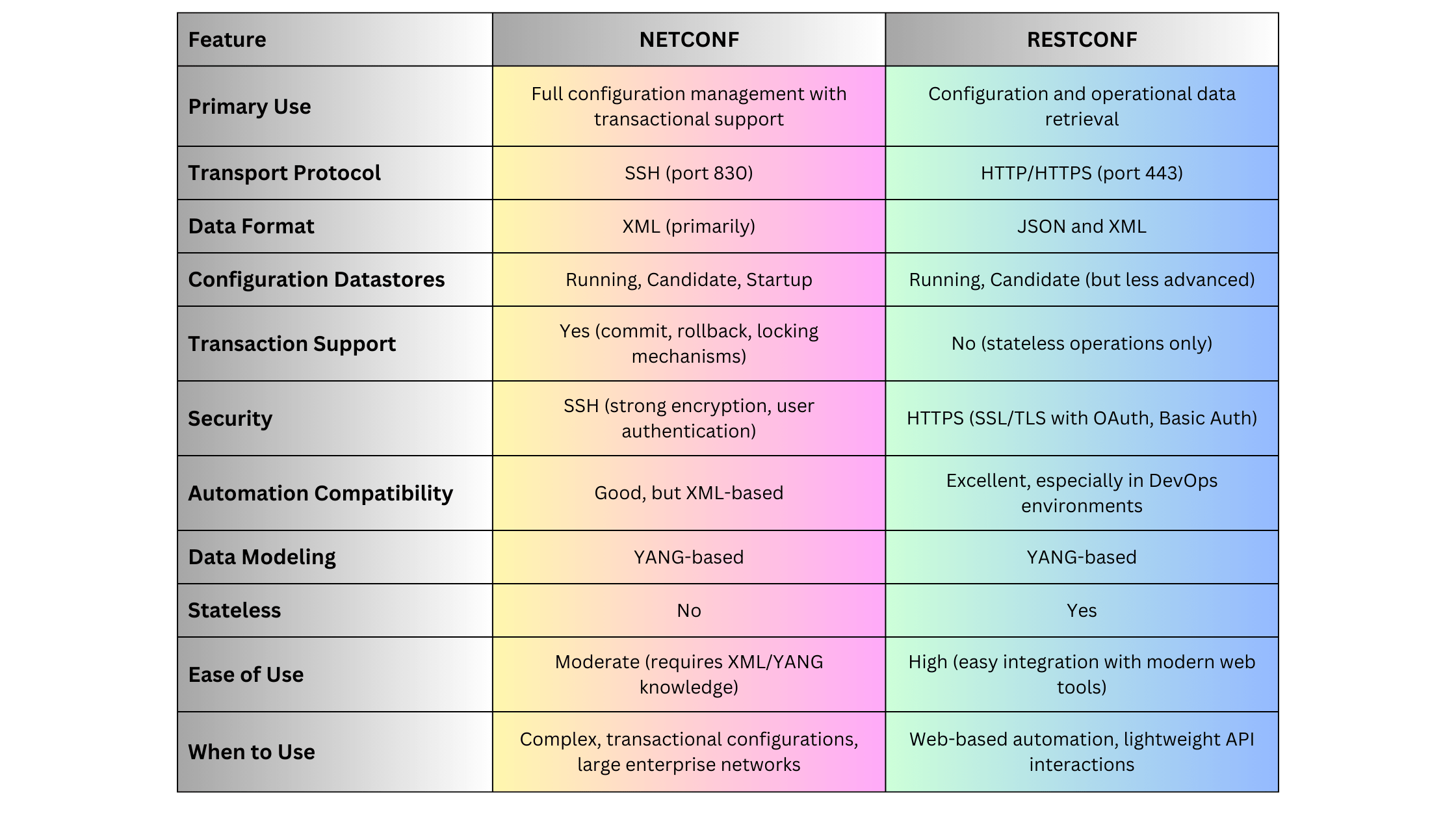
RESTCONF Implementation Steps
To implement RESTCONF, follow these general steps:
Step 1: Enable RESTCONF on Devices
Ensure your devices support RESTCONF and enable it. For example, on Cisco IOS XE, you can enable RESTCONF with:
restconf
Step 2: Send RESTCONF Requests
Once RESTCONF is enabled, you can interact with the device using curl or tools like Postman. For example, to retrieve the configuration of interfaces, you can use:
curl -k -u admin:admin "https://192.168.1.1:443/restconf/data/ietf-interfaces:interfaces"
Step 3: Parse JSON/XML Responses
RESTCONF responses will return data in JSON or XML format. If you’re using automation scripts (e.g., Python), you can parse this data to retrieve or modify configurations.
Summary
RESTCONF is a powerful, lightweight, and flexible protocol for managing network devices in a programmable way. Its use of HTTP/HTTPS, JSON, and YANG makes it a natural fit for web-based network automation tools and DevOps environments. While it lacks the transactional features of NETCONF, its simplicity and compatibility with modern APIs make it ideal for managing cloud-based and automated networks.
")
NETCONF (Network Configuration Protocol) is a modern protocol developed to address the limitations of older network management protocols like SNMP, especially for configuration management. It provides a robust, scalable, and secure method for managing network devices, supporting both configuration and operational data retrieval. NETCONF is widely used in modern networking environments, where automation, programmability, and fine-grained control are essential. Lets explore the NETCONF protocol, its architecture, advantages, use cases, security, and when to use it.
What Is NETCONF?
NETCONF (defined in RFC 6241) is a network management protocol that allows network administrators to install, manipulate, and delete the configuration of network devices. Unlike SNMP, which is predominantly used for monitoring, NETCONF focuses on configuration management and supports advanced features like transactional changes and candidate configuration models.
Key Features:
- Transaction-based Configuration: NETCONF allows administrators to make changes to network device configurations in a transactional manner, ensuring either full success or rollback in case of failure.
- Data Model Driven: NETCONF uses YANG (Yet Another Next Generation) as a data modeling language to define configuration and state data for network devices.
- Extensible and Secure: NETCONF is transport-independent and typically uses SSH (over port 830) to provide secure communication.
- Structured Data: NETCONF exchanges data in a structured XML format, ensuring clear, programmable access to network configurations and state information.
How NETCONF Works
NETCONF operates in a client-server architecture where the NETCONF client (usually a network management tool or controller) interacts with the NETCONF server (a network device) over a secure transport layer (commonly SSH). NETCONF performs operations like configuration retrieval, validation, modification, and state monitoring using a well-defined set of Remote Procedure Calls (RPCs).
NETCONF Workflow:
- Establish Session: The NETCONF client establishes a secure session with the device (NETCONF server), usually over SSH.
- Retrieve/Change Configuration: The client sends a <get-config> or <edit-config> RPC to retrieve or modify the device’s configuration.
- Transaction and Validation: NETCONF allows the use of a candidate configuration, where changes are made to a candidate datastore before committing to the running configuration, ensuring the changes are validated before they take effect.
- Apply Changes: Once validated, changes can be committed to the running configuration. If errors occur during the process, the transaction can be rolled back to a stable state.
- Close Session: After configuration changes are made or operational data is retrieved, the session can be closed securely.
NETCONF Operations
NETCONF supports a range of operations, defined as RPCs (Remote Procedure Calls), including:
- <get>: Retrieve device state information.
- <get-config>: Retrieve configuration data from a specific datastore (e.g., running, startup).
- <edit-config>: Modify the configuration data of a device.
- <copy-config>: Copy configuration data from one datastore to another.
- <delete-config>: Remove configuration data from a datastore.
- <commit>: Apply changes made in the candidate configuration to the running configuration.
- <lock> / <unlock>: Lock or unlock a configuration datastore to prevent conflicting changes.
These RPC operations allow network administrators to efficiently retrieve, modify, validate, and deploy configuration changes.
NETCONF Datastores
NETCONF supports different datastores for storing device configurations. The most common datastores are:
- Running Configuration: The current active configuration of the device.
- Startup Configuration: The configuration that is loaded when the device boots.
- Candidate Configuration: A working configuration area where changes can be tested before committing them to the running configuration.
The candidate configuration model provides a critical advantage over SNMP by enabling validation and rollback mechanisms before applying changes to the running state.
NETCONF and YANG
One of the key advantages of NETCONF is its tight integration with YANG, a data modeling language that defines the data structures used by network devices. YANG models provide a standardized way to represent device configurations and state information, ensuring interoperability between different devices and vendors.
YANG is essential for defining the structure of data that NETCONF manages, and it supports hierarchical data models that allow for more sophisticated and programmable interactions with network devices.
Security in NETCONF
NETCONF is typically transported over SSH (port 830), providing strong encryption and authentication for secure network device management. This is a significant improvement over SNMPv1 and SNMPv2c, which lack encryption and rely on clear-text community strings.
In addition to SSH, NETCONF can also be used with TLS (Transport Layer Security) or other secure transport layers, making it adaptable to high-security environments.
Advantages of NETCONF
NETCONF offers several advantages over legacy protocols like SNMP, particularly in the context of configuration management and network automation:
- Transaction-Based Configuration: NETCONF ensures that changes are applied in a transactional manner, reducing the risk of partial or incorrect configuration updates.
- YANG Model Integration: The use of YANG data models ensures structured, vendor-neutral device configuration, making automation easier and more reliable.
- Security: NETCONF uses secure transport protocols (SSH, TLS), protecting network management traffic from unauthorized access.
- Efficient Management: With support for retrieving and manipulating large configuration datasets in a structured format, NETCONF is highly efficient for managing modern, large-scale networks.
- Programmability: The structured XML or JSON data format and support for standardized YANG models make NETCONF highly programmable, ideal for software-defined networking (SDN) and network automation.
Disadvantages of NETCONF
Despite its many advantages, NETCONF does have some limitations:
- Complexity: NETCONF is more complex than SNMP, requiring an understanding of XML data structures and YANG models.
- Heavy Resource Usage: XML data exchanges are more verbose than SNMP’s simple GET/SET operations, potentially using more network and processing resources.
- Limited in Legacy Devices: Not all legacy devices support NETCONF, meaning a mix of protocols may need to be managed in hybrid environments.
When to Use NETCONF
NETCONF is best suited for large, modern networks where programmability, automation, and transactional configuration changes are required. Key use cases include:
- Network Automation: NETCONF is a foundational protocol for automating network configuration changes in software-defined networking (SDN) environments.
- Data Center Networks: Highly scalable and automated networks benefit from NETCONF’s structured configuration management.
- Cloud and Service Provider Networks: NETCONF is well-suited for multi-vendor environments where standardization and automation are necessary.
NETCONF vs. SNMP: A Quick Comparison
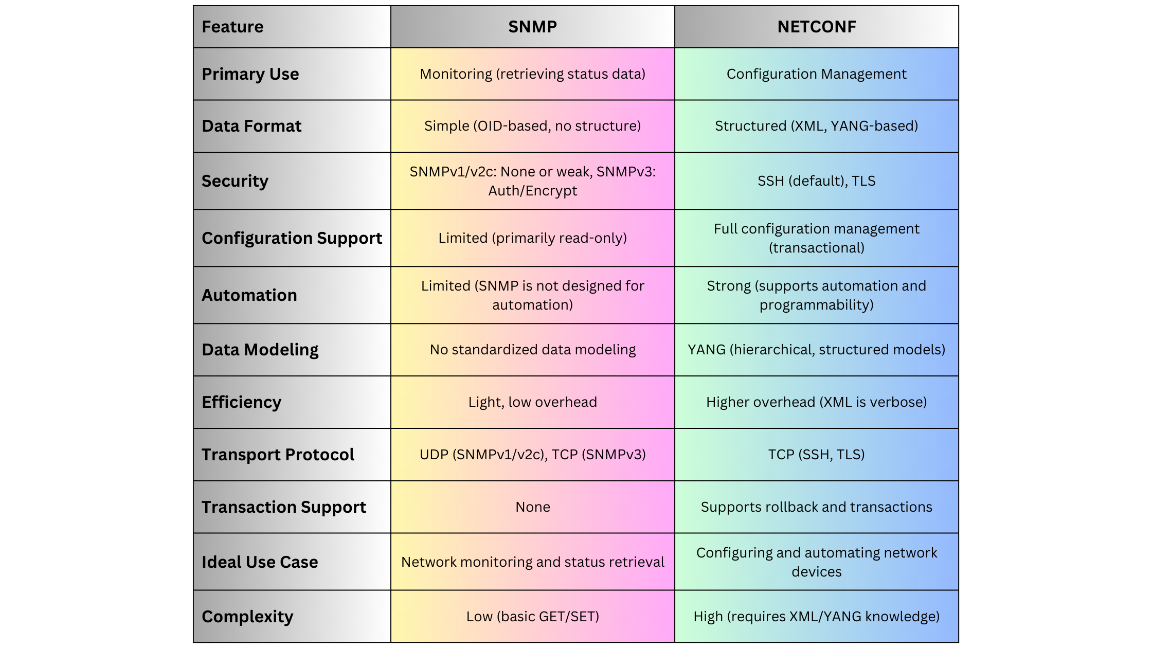
NETCONF Implementation Steps
Here is a general step-by-step process to implement NETCONF in a network:
Step 1: Enable NETCONF on Devices
Ensure that your network devices (routers, switches) support NETCONF and have it enabled. For example, on Cisco devices, this can be done with:
netconf sshStep 2: Install a NETCONF Client
To interact with devices, install a NETCONF client (e.g., ncclient in Python or Ansible modules that support NETCONF).
Step 3: Define the YANG Models
Identify the YANG models that are relevant to your device configurations. These models define the data structures NETCONF will manipulate.
Step 4: Retrieve or Edit Configuration
Use the <get-config> or <edit-config> RPCs to retrieve or modify device configurations. An example RPC call using Python’s ncclient might look like this:
from ncclient import manager

with manager.connect(host="192.168.1.1", port=830, username="admin", password="admin", hostkey_verify=False) as m:
    config = m.get_config(source='running')
    print(config)
Step 5: Validate and Commit Changes
Before applying changes, validate the configuration using <validate>, then commit it using <commit>.
Summary
NETCONF is a powerful, secure, and highly structured protocol for managing and automating network device configurations. Its tight integration with YANG data models and support for transactional configuration changes make it an essential tool for modern networks, particularly in environments where programmability and automation are critical. While more complex than SNMP, NETCONF provides the advanced capabilities necessary to manage large, scalable, and secure networks effectively.
Reference
")
Simple Network Management Protocol (SNMP) is one of the most widely used protocols for managing and monitoring network devices in IT environments. It allows network administrators to collect information, monitor device performance, and control devices remotely. SNMP plays a crucial role in the health, stability, and efficiency of a network, especially in large-scale or complex infrastructures. Let’s explore the ins and outs of SNMP, its various versions, key components, practical implementation, and how to leverage it effectively depending on network scale, complexity, and device type.
What Is SNMP?
SNMP stands for Simple Network Management Protocol, a standardized protocol used for managing and monitoring devices on IP networks. SNMP enables network devices such as routers, switches, servers, printers, and other hardware to communicate information about their state, performance, and errors to a centralized management system (SNMP manager).
Key Points:
- SNMP is an application layer protocol that operates on port 161 (UDP) for SNMP agent queries and port 162 (UDP) for SNMP traps.
- It is designed to simplify the process of gathering information from network devices and allows network administrators to perform remote management tasks, such as configuring devices, monitoring network performance, and troubleshooting issues.
How SNMP Works
SNMP consists of three main components:
- SNMP Manager: The management system that queries devices and collects data. It can be a network management software or platform, such as SolarWinds, PRTG, or Nagios.
- SNMP Agent: Software running on the managed device that responds to queries and sends traps (unsolicited alerts) to the SNMP manager.
- Management Information Base (MIB): A database of information that defines what can be queried or monitored on a network device. MIBs contain Object Identifiers (OIDs), which represent specific device metrics or configuration parameters.
The interaction between these components follows a request-response model:
- The SNMP manager sends a GET request to the SNMP agent to retrieve specific information.
- The agent responds with a GET response, containing the requested data.
- The SNMP manager can also send SET requests to modify configuration settings on the device.
- The SNMP agent can autonomously send TRAPs (unsolicited alerts) to notify the SNMP manager of critical events like device failure or threshold breaches.
SNMP Versions and Variants
SNMP has evolved over time, with different versions addressing various challenges related to security, scalability, and efficiency. The main versions are:
SNMPv1 (Simple Network Management Protocol Version 1)
-
- Introduction: The earliest version, released in the late 1980s, and still in use in smaller or legacy networks.
- Features: Provides basic management functions, but lacks robust security. Data is sent in clear text, which makes it vulnerable to eavesdropping.
- Use Case: Suitable for simple or isolated network environments where security is not a primary concern.
SNMPv2c (Community-Based SNMP Version 2)
-
- Introduction: Introduced to address some performance and functionality limitations of SNMPv1.
- Features: Improved efficiency with additional PDU types, such as GETBULK, which allows for the retrieval of large datasets in a single request. It still uses community strings (passwords) for security, which is minimal and lacks encryption.
- Use Case: Useful in environments where scalability and performance are needed, but without the strict need for security.
SNMPv3 (Simple Network Management Protocol Version 3)
-
- Introduction: Released to address security flaws in previous versions.
- Features:
-
-
-
-
- User-based Security Model (USM): Introduces authentication and encryption to ensure data integrity and confidentiality. Devices and administrators must authenticate using username/password, and messages can be encrypted using algorithms like AES or DES.
- View-based Access Control Model (VACM): Provides fine-grained access control to determine what data a user or application can access or modify.
- Security Levels: Three security levels: noAuthNoPriv, authNoPriv, and authPriv, offering varying degrees of security.
-
-
-
-
- Use Case: Ideal for large enterprise networks or any environment where security is a concern. SNMPv3 is now the recommended standard for new implementations.
SNMP Over TLS and DTLS
- Introduction: An emerging variant that uses Transport Layer Security (TLS) or Datagram Transport Layer Security (DTLS) to secure SNMP communication.
- Features: Provides better security than SNMPv3 in some contexts by leveraging more robust transport layer encryption.
- Use Case: Suitable for modern, security-conscious organizations where protecting management traffic is a priority.
SNMP Communication Example
Here’s a basic example of how SNMP operates in a typical network as a reference for readers:
Scenario: A network administrator wants to monitor the CPU usage of a optical device.
- Step 1: The SNMP manager sends a GET request to the SNMP agent on the optical device to query its CPU usage. The request contains the OID corresponding to the CPU metric (e.g., .1.3.6.1.4.1.9.2.1.57 for Optical devices).
- Step 2: The SNMP agent on the optical device retrieves the requested data from its MIB and responds with a GET response containing the CPU usage percentage.
- Step 3: If the CPU usage exceeds a defined threshold, the SNMP agent can autonomously send a TRAP message to the SNMP manager, alerting the administrator of the high CPU usage.
SNMP Message Types
SNMP uses several message types, also known as Protocol Data Units (PDUs), to facilitate communication between the SNMP manager and the agent:
- GET: Requests information from the SNMP agent.
- GETNEXT: Retrieves the next value in a table or list.
- SET: Modifies the value of a device parameter.
- GETBULK: Retrieves large amounts of data in a single request (introduced in SNMPv2).
- TRAP: A notification from the agent to the manager about significant events (e.g., device failure).
- INFORM: Similar to a trap, but includes an acknowledgment mechanism to ensure delivery (introduced in SNMPv2).
SNMP MIBs and OIDs
The Management Information Base (MIB) is a structured database of information that defines what aspects of a device can be monitored or controlled. MIBs use a hierarchical structure defined by Object Identifiers (OIDs).
- OIDs: OIDs are unique identifiers that represent individual metrics or device properties. They follow a dotted-decimal format and are structured hierarchically.
- Example: The OID .1.3.6.1.2.1.1.5.0 refers to the system name of a device.
Advantages of SNMP
SNMP provides several advantages for managing network devices:
- Simplicity: SNMP is easy to implement and use, especially for small to medium-sized networks.
- Scalability: With the introduction of SNMPv2c and SNMPv3, the protocol can handle large-scale network infrastructures by using bulk operations and secure communications.
- Automation: SNMP can automate the monitoring of thousands of devices, reducing the need for manual intervention.
- Cross-vendor Support: SNMP is widely supported across networking hardware and software, making it compatible with devices from different vendors (e.g., Ribbon, Cisco, Ciena, Nokia, Juniper, Huawei).
- Cost-Effective: Since SNMP is an open standard, it can be used without additional licensing costs, and many open-source SNMP management tools are available.
Disadvantages and Challenges
Despite its widespread use, SNMP has some limitations:
- Security: Early versions (SNMPv1, SNMPv2c) lacked strong security features, making them vulnerable to attacks. Only SNMPv3 introduces robust authentication and encryption.
- Complexity in Large Networks: In very large or complex networks, managing MIBs and OIDs can become cumbersome. Bulk data retrieval (GETBULK) helps, but can still introduce overhead.
- Polling Overhead: SNMP polling can generate significant traffic in very large environments, especially when retrieving large amounts of data frequently.
When to Use SNMP
The choice of SNMP version and its usage depends on the scale, complexity, and security requirements of the network:
Small Networks
-
Use SNMPv1 or SNMPv2c if security is not a major concern and simplicity is valued. These versions are easy to configure and work well in isolated environments where data is collected over a trusted network.
Medium to Large Networks
-
Use SNMPv2c for better efficiency and performance, especially when monitoring a large number of devices. GETBULK allows efficient retrieval of large datasets, reducing polling overhead. -
Implement SNMPv3 for environments where security is paramount. The encryption and authentication provided by SNMPv3 ensure that sensitive information (e.g., passwords, configuration changes) is protected from unauthorized access.
Highly Secure Networks
-
Use SNMPv3 or SNMP over TLS/DTLS in networks that require the highest level of security (e.g., financial services, government, healthcare). These environments benefit from robust encryption, authentication, and access control mechanisms provided by these variants.
Implementation Steps
Implementing SNMP in a network requires careful planning, especially when using SNMPv3:
Step 1: Device Configuration
- Enable SNMP on devices: For each device (e.g., switch, router), enable the appropriate SNMP version and configure the SNMP agent.
- For SNMPv1/v2c: Define a community string (password) to restrict access to SNMP data.
- For SNMPv3: Configure users, set security levels, and enable encryption.
Step 2: SNMP Manager Setup
- Install SNMP management software such as PRTG, Nagios, MGSOFT or SolarWinds. Configure it to monitor the devices and specify the correct SNMP version and credentials.
Step 3: Define MIBs and OIDs
- Import device-specific MIBs to allow the SNMP manager to understand the device’s capabilities. Use OIDs to monitor or control specific metrics like CPU usage, memory, or bandwidth.
Step 4: Monitor and Manage Devices
- Set up regular polling intervals and thresholds for key metrics. Configure SNMP traps to receive immediate alerts for critical events.
SNMP Trap Example
To illustrate the use of SNMP traps, consider a situation where a router’s interface goes down:
- The SNMP agent on the router detects the interface failure.
- It immediately sends a TRAP message to the SNMP manager.
- The SNMP manager receives the TRAP and notifies the network administrator about the failure.
Practical Example of SNMP GET Request
Let’s take an example of using SNMP to query the system uptime from a device:
- OID for system uptime: .1.3.6.1.2.1.1.3.0
- SNMP Command: To query the uptime using the command-line tool snmpget:
snmpget -v2c -c public 192.168.1.1 .1.3.6.1.2.1.1.3.0Here,
-v2c specifies SNMPv2c,

-c public specifies the community string,

192.168.1.1 is the IP of the SNMP-enabled device, and

.1.3.6.1.2.1.1.3.0 is the OID for the system uptime.
DISMAN-EVENT-MIB::sysUpTimeInstance = Timeticks: (5321) 0:00:53.21SNMP Alternatives
Although SNMP is widely used, there are other network management protocols available. Some alternatives include:
- NETCONF: A newer protocol designed for network device configuration, with a focus on automating complex tasks.
- RESTCONF: A RESTful API-based protocol used to configure and monitor network devices.
- gNMI (gRPC Network Management Interface): An emerging standard for telemetry and control, designed for modern networks and cloud-native environments.
Summary
SNMP is a powerful tool for monitoring and managing network devices across small, medium, and large-scale networks. Its simplicity, wide adoption, and support for cross-vendor hardware make it an industry standard for network management. However, network administrators should carefully select the appropriate SNMP version depending on the security and scalability needs of their environment. SNMPv3 is the preferred choice for modern networks due to its strong authentication and encryption features, ensuring that network management traffic is secure.
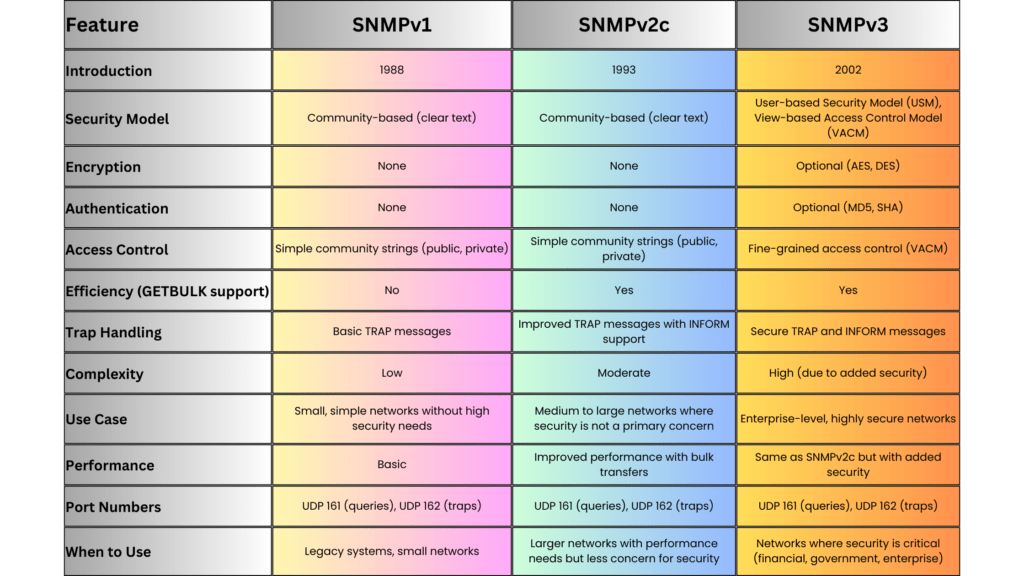
 in DWDM Networks")
Stimulated Brillouin Scattering (SBS) is an inelastic scattering phenomenon that results in the backward scattering of light when it interacts with acoustic phonons (sound waves) in the optical fiber. SBS occurs when the intensity of the optical signal reaches a certain threshold, resulting in a nonlinear interaction between the optical field and acoustic waves within the fiber. This effect typically manifests at lower power levels compared to other nonlinear effects, making it a significant limiting factor in optical communication systems, particularly those involving long-haul transmission and high-power signals.
Mechanism of SBS
SBS is caused by the interaction of an incoming photon with acoustic phonons in the fiber material. When the intensity of the light increases beyond a certain threshold, the optical signal generates an acoustic wave in the fiber. This acoustic wave, in turn, causes a periodic variation in the refractive index of the fiber, which scatters the incoming light in the backward direction. This backscattered light is redshifted in frequency due to the Doppler effect, with the frequency shift typically around 10 GHz (depending on the fiber material and the wavelength of light).
The Brillouin gain spectrum is relatively narrow, with a typical bandwidth of around 20 to 30 MHz. The Brillouin threshold power can be calculated as:
Where:
- is the effective area of the fiber core,
- is the Brillouin gain coefficient,
- is the effective interaction length of the fiber.
When the power of the incoming light exceeds this threshold, SBS causes a significant amount of power to be reflected back towards the source, degrading the forward-propagating signal and introducing power fluctuations in the system.
Image credit: corning.com
Impact of SBS in Optical Systems
SBS becomes problematic in systems where high optical powers are used, particularly in long-distance transmission systems and those employing Wavelength Division Multiplexing (WDM). The main effects of SBS include:
- Power Reflection:
- A portion of the optical power is scattered back towards the source, which reduces the forward-propagating signal power. This backscattered light interferes with the transmitter and receiver, potentially causing signal degradation.
- Signal Degradation:
- SBS can cause signal distortion, as the backward-propagating light interferes with the incoming signal, leading to fluctuations in the transmitted power and an increase in the bit error rate (BER).
- Noise Increase:
- The backscattered light adds noise to the system, particularly in coherent systems, where phase information is critical. The interaction between the forward and backward waves can distort the phase and amplitude of the transmitted signal, worsening the signal-to-noise ratio (SNR).
SBS in Submarine Systems
In submarine communication systems, SBS poses a significant challenge, as these systems typically involve long spans of fiber and require high power levels to maintain signal quality over thousands of kilometers. The cumulative effect of SBS over long distances can lead to substantial signal degradation. As a result, submarine systems must employ techniques to suppress SBS and manage the power levels appropriately.
Mitigation Techniques for SBS
Several methods are used to mitigate the effects of SBS in optical communication systems:
- Reducing Signal Power:
- One of the simplest ways to reduce the onset of SBS is to lower the optical signal power below the Brillouin threshold. However, this must be balanced with maintaining sufficient power for the signal to reach its destination with an acceptable signal-to-noise ratio (SNR).
- Laser Linewidth Broadening:
- SBS is more efficient when the signal has a narrow linewidth. By broadening the linewidth of the signal, the power is spread over a larger frequency range, reducing the power density at any specific frequency and lowering the likelihood of SBS. This can be achieved by modulating the laser source with a low-frequency signal.
- Using Shorter Fiber Spans:
- Reducing the length of each fiber span in the transmission system can decrease the effective length over which SBS can occur. By using optical amplifiers to boost the signal power at regular intervals, it is possible to maintain signal strength without exceeding the SBS threshold.
- Raman Amplification:
- SBS can be suppressed using distributed Raman amplification, where the signal is amplified along the length of the fiber rather than at discrete points. By keeping the power levels low in any given section of the fiber, Raman amplification reduces the risk of SBS.
Applications of SBS
While SBS is generally considered a detrimental effect in optical communication systems, it can be harnessed for certain useful applications:
- Brillouin-Based Sensors:
- SBS is used in distributed fiber optic sensors, such as Brillouin Optical Time Domain Reflectometry (BOTDR) and Brillouin Optical Time Domain Analysis (BOTDA). These sensors measure the backscattered Brillouin light to monitor changes in strain or temperature along the length of the fiber. This is particularly useful in structural health monitoring and pipeline surveillance.
- Slow Light Applications:
- SBS can also be exploited to create slow light systems, where the propagation speed of light is reduced in a controlled manner. This is achieved by using the narrow bandwidth of the Brillouin gain spectrum to induce a delay in the transmission of the optical signal. Slow light systems have potential applications in optical buffering and signal processing.
Summary
Stimulated Brillouin Scattering (SBS) is a nonlinear scattering effect that occurs at relatively low power levels, making it a significant limiting factor in high-power, long-distance optical communication systems. SBS leads to the backscattering of light, which degrades the forward-propagating signal and increases noise. While SBS is generally considered a negative effect, it can be mitigated using techniques such as power reduction, linewidth broadening, and Raman amplification. Additionally, SBS can be harnessed for beneficial applications, including optical sensing and slow light systems. Effective management of SBS is crucial for maintaining the performance and reliability of modern optical communication networks, particularly in submarine systems.
- Stimulated Brillouin Scattering (SBS) is a nonlinear optical effect caused by the interaction between light and acoustic waves in the fiber.
- It occurs when an intense light wave traveling through the fiber generates sound waves, which scatter the light in the reverse direction.
- SBS leads to a backward-propagating signal, called the Stokes wave, that has a slightly lower frequency than the incoming light.
- The effect typically occurs in single-mode fibers at relatively low power thresholds compared to other nonlinear effects like SRS.
- SBS can result in power loss of the forward-propagating signal as some of the energy is reflected back as the Stokes wave.
- The efficiency of SBS depends on several factors, including the fiber length, the optical power, and the linewidth of the laser source.
- In WDM systems, SBS can degrade performance by introducing signal reflections and crosstalk, especially in long-haul optical links.
- SBS tends to become more pronounced in narrow-linewidth lasers and fibers with low attenuation, making it a limiting factor for high-power transmission.
- Mitigation techniques for SBS include using broader linewidth lasers, reducing the optical power below the SBS threshold, or employing SBS suppression techniques such as phase modulation.
- Despite its negative impacts in communication systems, SBS can be exploited for applications like distributed fiber sensing and slow-light generation due to its sensitivity to acoustic waves.
Reference
 in DWDM Networks")
Stimulated Raman Scattering (SRS) is a nonlinear optical phenomenon that results from the inelastic scattering of photons when intense light interacts with the vibrational modes of the fiber material. This scattering process transfers energy from shorter-wavelength (higher-frequency) channels to longer-wavelength (lower-frequency) channels. In fiber optic communication systems, particularly in Wavelength Division Multiplexing (WDM) systems, SRS can significantly degrade system performance by inducing crosstalk between channels.
Physics behind SRS
SRS is an inelastic process involving the interaction of light photons with the optical phonons (vibrational states) of the silica material in the fiber. When a high-power optical signal propagates through the fiber, a fraction of the power is scattered by the material, transferring energy from the higher frequency (shorter wavelength) channels to the lower frequency (longer wavelength) channels. The SRS gain is distributed over a wide spectral range, approximately 13 THz, with a peak shift of about 13.2 THz from the pump wavelength.
The basic process of SRS can be described as follows:
- Stokes Shift: The scattered light is redshifted, meaning that the scattered photons have lower energy (longer wavelength) than the incident photons. This energy loss is transferred to the vibrational modes (phonons) of the fiber.
- Amplification: The power of longer-wavelength channels is increased at the expense of shorter-wavelength channels. This power transfer can cause crosstalk between channels in WDM systems, reducing the overall signal quality.
Fig: Normalized gain spectrum generated by SRS on an SSMF fiber pumped at 1430 nm. The SRS gain spectrum has a peak at 13 THz with a bandwidth of 20–30 THz
The Raman gain coefficient describes the efficiency of the SRS process and is dependent on the frequency shift and the fiber material. The Raman gain spectrum is typically broad, extending over several terahertz, with a peak at a frequency shift of around 13.2 THz.
Mathematical Representation
The Raman gain coefficient varies with the wavelength and fiber properties. The SRS-induced power tilt between channels can be expressed using the following relation:
Where:
- is the effective length of the fiber,
- is the effective core area of the fiber,
- is the output power,
- is the wavelength bandwidth of the signal.
This equation shows that the magnitude of the SRS effect depends on the effective length, core area, and wavelength separation. Higher power, larger bandwidth, and longer fibers increase the severity of SRS.
Impact of SRS in WDM Systems
In WDM systems, where multiple wavelengths are transmitted simultaneously, SRS leads to a power transfer from shorter-wavelength channels to longer-wavelength channels. The main effects of SRS in WDM systems include:
- Crosstalk:
-
-
-
-
-
- SRS causes power from higher-frequency channels to be transferred to lower-frequency channels, leading to crosstalk between WDM channels. This degrades the signal quality, particularly for channels with lower frequencies, which gain excess power, while higher-frequency channels experience a power loss.
-
-
-
-
-
- Channel Degradation:
-
-
-
-
- The unequal power distribution caused by SRS degrades the signal-to-noise ratio (SNR) of individual channels, particularly in systems with closely spaced WDM channels. This results in increased bit error rates (BER) and degraded overall system performance.
-
-
-
-
- Signal Power Tilt:
-
-
-
-
- SRS induces a power tilt across the WDM spectrum, with lower-wavelength channels losing power and higher-wavelength channels gaining power. This tilt can be problematic in systems where precise power levels are critical for maintaining signal integrity.
-
-
-
-
SRS in Submarine Systems
SRS plays a significant role in submarine optical communication systems, where long transmission distances and high power levels make the system more susceptible to nonlinear effects. In ultra-long-haul submarine systems, SRS-induced crosstalk can accumulate over long distances, degrading the overall system performance. To mitigate this, submarine systems often employ Raman amplification techniques, where the SRS effect is used to amplify the signal rather than degrade it.
Mitigation Techniques for SRS
Several techniques can be employed to mitigate the effects of SRS in optical communication systems:
- Channel Spacing:
-
-
-
-
- Increasing the spacing between WDM channels reduces the interaction between the channels, thereby reducing the impact of SRS. However, this reduces spectral efficiency and limits the number of channels that can be transmitted.
-
-
-
-
- Power Optimization:
-
-
-
-
- Reducing the launch power of the optical signals can limit the onset of SRS. However, this must be balanced with maintaining adequate signal power for long-distance transmission.
-
-
-
-
- Raman Amplification:
-
-
-
-
- SRS can be exploited in distributed Raman amplification systems, where the scattered Raman signal is used to amplify longer-wavelength channels. By carefully controlling the pump power, SRS can be harnessed to improve system performance rather than degrade it.
-
-
-
-
- Gain Flattening Filters:
-
-
-
-
- Gain-flattening filters can be used to equalize the power levels of WDM channels after they have been affected by SRS. These filters counteract the power tilt induced by SRS and restore the balance between channels.
-
-
-
-
Applications of SRS
Despite its negative impact on WDM systems, SRS can be exploited for certain beneficial applications, particularly in long-haul and submarine systems:
- Raman Amplification:
-
-
-
-
- Raman amplifiers use the SRS effect to amplify optical signals in the transmission fiber. By injecting a high-power pump signal into the fiber, the SRS process can be used to amplify the lower-wavelength signal channels, extending the reach of the system.
-
-
-
-
- Signal Regeneration:
-
-
-
-
- SRS can be used in all-optical regenerators, where the Raman scattering effect is used to restore the signal power and quality in long-haul systems.
-
-
-
-
Summary
Stimulated Raman Scattering (SRS) is a critical nonlinear effect in optical fiber communication, particularly in WDM and submarine systems. It results in the transfer of power from higher-frequency to lower-frequency channels, leading to crosstalk and power imbalance. While SRS can degrade system performance, it can also be harnessed for beneficial applications such as Raman amplification. Proper management of SRS is essential for optimizing the capacity and reach of modern optical communication systems, especially in ultra-long-haul and submarine networks
- Stimulated Raman Scattering (SRS) is a nonlinear effect that occurs when high-power light interacts with the fiber material, transferring energy from shorter-wavelength (higher-frequency) channels to longer-wavelength (lower-frequency) channels.
- SRS occurs due to the inelastic scattering of photons, which interact with the vibrational states of the fiber material, leading to energy redistribution between wavelengths.
- The SRS effect results in power being transferred from higher-frequency channels to lower-frequency channels, causing signal crosstalk and potential degradation.
- The efficiency of SRS depends on the Raman gain coefficient, fiber length, power levels, and wavelength spacing.
- SRS can induce signal degradation in WDM systems, leading to power imbalances and increased bit error rates (BER).
- In submarine systems, SRS plays a significant role in long-haul transmissions, as it accumulates over long distances, further degrading signal quality.
- Techniques like increasing channel spacing, optimizing signal power, and using Raman amplification can mitigate SRS.
- Raman amplification, which is based on the SRS effect, can be used beneficially to boost signals over long distances.
- Gain-flattening filters are used to balance the power across wavelengths affected by SRS, improving overall system performance.
- SRS is particularly significant in long-haul optical systems but can also be harnessed for signal regeneration and amplification in modern optical communication systems.
Reference
- https://link.springer.com/book/10.1007/978-3-030-66541-8
- Image : https://link.springer.com/book/10.1007/978-3-030-66541-8 (SRS)
 in DWDM Networks")
Four-Wave Mixing (FWM) is a nonlinear optical phenomenon that occurs when multiple wavelengths of light are transmitted through a fiber simultaneously. FWM is a third-order nonlinear effect, and it results in the generation of new wavelengths (or frequencies) through the interaction of the original light waves. It is one of the most important nonlinear effects in Wavelength Division Multiplexing (WDM) systems, where multiple wavelength channels are used to increase the system capacity.
Physics behind FWM
FWM occurs when three optical waves, at frequencies 𝑓1,𝑓2 and 𝑓3, interact in the fiber to produce a fourth wave at a frequency 𝑓4, which is generated by the nonlinear interaction between the original waves. The frequency of the new wave is given by:
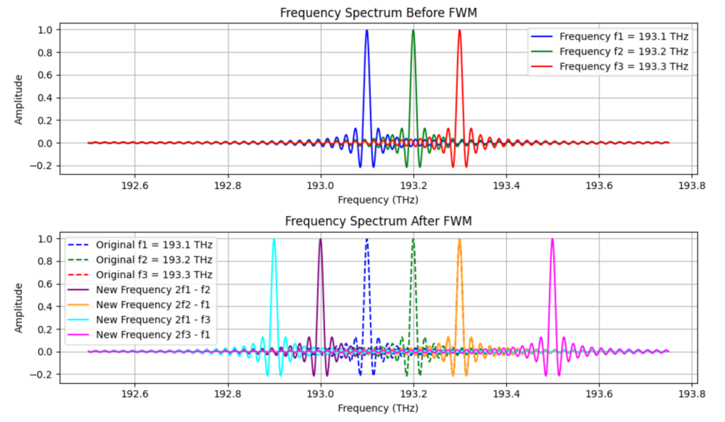 This process is often referred to as third-order intermodulation, where new frequencies are created due to the mixing of the input signals. For FWM to be efficient, the interacting waves must satisfy certain phase-matching conditions, which depend on the chromatic dispersion and the effective refractive index of the fiber.
Mathematical Expression
The general formula for FWM efficiency can be expressed as:
Where:
- 𝑃FWM is the power of the generated FWM signal.
- 𝑃1,𝑃2,𝑃3 are the powers of the interacting signals.
- 𝜂 is the FWM efficiency factor which depends on the fiber’s chromatic dispersion, the effective area, and the nonlinear refractive index.
The efficiency of FWM is highly dependent on the phase-matching condition, which is affected by the chromatic dispersion of the fiber. If the fiber has zero or low dispersion, FWM becomes more efficient, and more power is transferred to the new wavelengths. Conversely, in fibers with higher dispersion, FWM is less efficient.
Impact of FWM in WDM Systems
FWM has a significant impact in WDM systems, particularly when the channel spacing between the wavelengths is narrow. The main effects of FWM include:
- Crosstalk:
-
-
-
-
- FWM generates new frequencies that can interfere with the original WDM channels, leading to crosstalk between channels. This crosstalk can degrade the signal quality, especially when the system operates with high power and closely spaced channels.
-
-
-
-
- Spectral Efficiency:
-
-
-
-
- FWM can limit the spectral efficiency of the system by introducing unwanted signals in the spectrum. This imposes a practical limit on how closely spaced the WDM channels can be, as reducing the channel spacing increases the likelihood of FWM.
-
-
-
-
- Performance Degradation:
-
-
-
-
- The new frequencies generated by FWM can overlap with the original signal channels, leading to increased bit error rates (BER) and reduced signal-to-noise ratios (SNR). This is particularly problematic in long-haul optical systems, where FWM accumulates over long distances.
-
-
-
-
FWM and Chromatic Dispersion
Chromatic dispersion plays a critical role in the occurrence of FWM. Dispersion-managed fibers can be designed to control the effects of FWM by increasing the phase mismatch between the interacting waves, thereby reducing FWM efficiency. In contrast, fibers with zero-dispersion wavelengths can significantly enhance FWM, as the phase-matching condition is more easily satisfied.
In practical systems, fibers with non-zero dispersion-shifted fibers (NZDSF) are often used to reduce the impact of FWM. NZDSF fibers have a dispersion profile that is designed to keep the system out of the zero-dispersion regime while minimizing the dispersion penalty.
Mitigation Techniques for FWM
Several techniques can be employed to mitigate the effects of FWM in optical communication systems:
- Increase Channel Spacing:By increasing the channel spacing between WDM signals, the interaction between channels is reduced, thereby minimizing FWM. However, this reduces the overall capacity of the system.
- Optimize Power Levels:Reducing the launch power of the optical signals can lower the nonlinear interaction and reduce the efficiency of FWM. However, this must be balanced with maintaining sufficient optical power to achieve the desired signal-to-noise ratio (SNR).
- Use Dispersion-Managed Fibers: As mentioned above, fibers with optimized dispersion profiles can be used to reduce the efficiency of FWM by increasing the phase mismatch between interacting wavelengths.
- Employ Advanced Modulation Formats:Modulation formats that are less sensitive to phase distortions, such as differential phase-shift keying (DPSK), can help reduce the impact of FWM on signal quality.
- Optical Phase Conjugation:Optical phase conjugation can be used to counteract the effects of FWM by reversing the nonlinear phase distortions. This technique is typically implemented in mid-span spectral inversion systems, where the phase of the signal is conjugated at a point in the transmission link.
Applications of FWM
Despite its negative impact on WDM systems, FWM can also be exploited for useful applications:
- Wavelength Conversion:
- FWM can be used for all-optical wavelength conversion, where the interacting wavelengths generate a new wavelength that can be used for wavelength routing or switching in WDM networks.
- Signal Regeneration:
- FWM has been used in all-optical regenerators, where the nonlinear interaction between signals is used to regenerate the optical signal, improving its quality and extending the transmission distance.
FWM in Submarine Systems
In submarine optical communication systems, where long-distance transmission is required, FWM poses a significant challenge. The accumulation of FWM over long distances can lead to severe crosstalk and signal degradation. Submarine systems often use large effective area fibers to reduce the nonlinear interactions and minimize FWM. Additionally, dispersion management is employed to limit the efficiency of FWM by introducing phase mismatch between the interacting waves.
Summary
Four-Wave Mixing (FWM) is a critical nonlinear effect in optical fiber communication, particularly in WDM systems. It leads to the generation of new wavelengths, causing crosstalk and performance degradation. Managing FWM is essential for optimizing the capacity and reach of optical systems, particularly in long-haul and submarine communication networks. Techniques such as dispersion management, power optimization, and advanced modulation formats can help mitigate the effects of FWM and improve the overall system performance.
- Four-Wave Mixing (FWM) is a nonlinear optical effect that occurs when multiple wavelengths of light travel through a fiber, generating new frequencies from the original signals.
- It’s a third-order nonlinear phenomenon and is significant in Wavelength Division Multiplexing (WDM) systems, where it can affect system capacity.
- FWM happens when three optical waves interact to create a fourth wave, and its efficiency depends on the phase-matching condition, which is influenced by chromatic dispersion.
- The formula for FWM efficiency depends on the power of the interacting signals and the FWM efficiency factor, which is impacted by the fiber’s dispersion and other parameters.
- FWM can cause crosstalk in WDM systems by generating new frequencies that interfere with the original channels, degrading signal quality.
- It reduces spectral efficiency by limiting how closely WDM channels can be spaced due to the risk of FWM.
- FWM can lead to performance degradation in optical systems, especially over long distances, increasing error rates and lowering the signal-to-noise ratio (SNR).
- Managing chromatic dispersion in fibers can reduce FWM’s efficiency, with non-zero dispersion-shifted fibers often used to mitigate the effect.
- Techniques to reduce FWM include increasing channel spacing, optimizing power levels, using dispersion-managed fibers, and employing advanced modulation formats.
- Despite its negative impacts, FWM can be useful for wavelength conversion and signal regeneration in certain optical applications, and it is a challenge in long-distance submarine systems.
Reference
- https://link.springer.com/book/10.1007/978-3-030-66541-8
 in DWDM Networks")
Cross-Phase Modulation (XPM) is a nonlinear effect that occurs in Wavelength Division Multiplexing (WDM) systems. It is a type of Kerr effect, where the intensity of one optical signal induces phase shifts in another signal traveling through the same fiber. XPM arises when multiple optical signals of different wavelengths interact, causing crosstalk between channels, leading to phase distortion and signal degradation.
Physics behind XPM
In XPM, the refractive index of the fiber is modulated by the intensity fluctuations of different signals. When multiple wavelengths propagate through a fiber, the intensity variations of each signal affect the phase of the other signals through the Kerr nonlinearity:
Where:
- n0 is the linear refractive index.
- 𝑛2 is the nonlinear refractive index coefficient.
- 𝐼 is the intensity of the light signal.
XPM occurs because the intensity fluctuations of one channel change the refractive index of the fiber, which in turn alters the phase of the other channels. The phase modulation imparted on the affected channel is proportional to the power of the interfering channels.
The phase shift Δϕ experienced by a signal due to XPM can be expressed as:
Where:
- γ is the nonlinear coefficient.
- P is the power of the interfering channel.
- Leff is the effective length of the fiber.
Mathematical Representation
The total impact of XPM can be described by the Nonlinear Schrödinger Equation (NLSE), where the nonlinear term accounts for both SPM (Self-Phase Modulation) and XPM. The nonlinear term for XPM can be included as follows:
Where:
- A is the complex field of the signal.
- 𝛽2 represents group velocity dispersion.
- 𝛾 is the nonlinear coefficient.
In WDM systems, this equation must consider the intensity of other signals:
Where the summation accounts for the impact of all interfering channels.
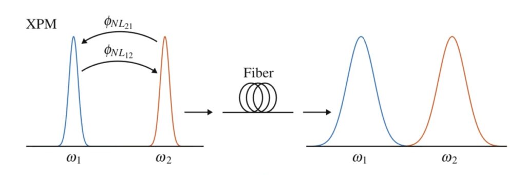
Fig: In XPM, amplitude variations of a signal in frequency ω1 (or ω2) generate a pattern-dependent nonlinear phase shift φNL12 (or φNL21 ) on a second signal of frequency ω2 (or ω1), causing spectral broadening and impairing transmission
Effects of XPM
- Crosstalk Between Wavelengths: XPM introduces crosstalk between different wavelength channels in WDM systems. The intensity fluctuations of one channel induce phase modulation in the other channels, leading to signal degradation and noise.
- Interference: Since the phase of a channel is modulated by the power of other channels, XPM leads to inter-channel interference, which degrades the signal-to-noise ratio (SNR) and increases the bit error rate (BER).
- Spectral Broadening: XPM can cause broadening of the signal spectrum, similar to the effects of Self-Phase Modulation (SPM). This broadening worsens chromatic dispersion, leading to pulse distortion.
- Pattern Dependence: XPM is pattern-dependent, meaning that the phase distortion introduced by XPM depends on the data patterns in the neighboring channels. This can cause significant performance degradation, particularly in systems using phase-sensitive modulation formats like QPSK or QAM.
XPM in Coherent Systems
In coherent optical communication systems, which use digital signal processing (DSP), the impact of XPM can be mitigated to some extent. Coherent systems detect both the phase and amplitude of the signal, allowing for more efficient compensation of phase distortions caused by XPM. However, even in coherent systems, XPM still imposes limitations on transmission distance and system capacity.
Impact of Dispersion on XPM
Chromatic dispersion plays a crucial role in the behavior of XPM. In fibers with low dispersion, XPM effects are stronger because the interacting signals travel at similar group velocities, increasing their interaction length. However, in fibers with higher dispersion, the signals experience walk-off, where they travel at different speeds, reducing the impact of XPM through an averaging effect.
Dispersion management is often used to mitigate XPM in long-haul systems by ensuring that the interacting signals separate spatially as they propagate through the fiber, reducing the extent of their interaction.
Mitigation Techniques for XPM
Several techniques are used to mitigate the impact of XPM in optical systems:
- Increase Channel Spacing:
- Increasing the spacing between wavelength channels in WDM systems reduces the likelihood of XPM-induced crosstalk. However, this reduces spectral efficiency, limiting the total number of channels that can be transmitted.
- Optimizing Power Levels:
- Reducing the launch power of the signals can limit the nonlinear phase shift caused by XPM. However, this must be balanced with maintaining an adequate signal-to-noise ratio (SNR).
- Dispersion Management:
- By carefully managing chromatic dispersion in the fiber, it is possible to reduce the interaction between different channels, thereby mitigating XPM. This is often achieved by using dispersion-compensating fibers or digital signal processing (DSP).
- Advanced Modulation Formats:
- Using modulation formats that are less sensitive to phase distortions, such as differential phase-shift keying (DPSK), can reduce the impact of XPM on the signal.
Applications of XPM
While XPM generally has a negative impact on system performance, it can be exploited for certain applications:
- Wavelength Conversion:
- XPM can be used for all-optical wavelength conversion in WDM systems. The phase modulation caused by one signal can be used to shift the wavelength of another signal, allowing for dynamic wavelength routing in optical networks.
- Nonlinear Signal Processing:
- XPM can be used in nonlinear signal processing techniques, where the nonlinear phase shifts induced by XPM are used for signal regeneration, clock recovery, or phase modulation.
XPM in Submarine Systems
In ultra-long-haul submarine systems, XPM is a significant limiting factor for system performance. Submarine systems typically use dense wavelength division multiplexing (DWDM), where the close spacing between channels exacerbates the effects of XPM. To mitigate this, submarine systems employ dispersion management, low-power transmission, and advanced digital signal processing techniques to counteract the phase distortion caused by XPM.
Summary
Cross-Phase Modulation (XPM) is a critical nonlinear effect in WDM systems, where the intensity fluctuations of one wavelength channel modulate the phase of other channels. XPM leads to inter-channel crosstalk, phase distortion, and spectral broadening, which degrade system performance. Managing XPM is essential for optimizing the capacity and reach of modern optical communication systems, particularly in coherent systems and submarine cable networks. Proper dispersion management, power optimization, and advanced modulation formats can help mitigate the impact of XPM.
- Cross-Phase Modulation (XPM) is a nonlinear optical effect where the phase of a signal is influenced by the intensity of another signal in the same fiber.
- It happens in systems where multiple channels of light travel through the same optical fiber, such as in Dense Wavelength Division Multiplexing (DWDM) systems.
- XPM occurs because the light signals interact with each other through the fiber’s nonlinear properties, causing changes in the phase of the signals.
- The phase shift introduced by XPM leads to signal distortion and can affect the performance of communication systems by degrading the quality of the transmitted signals.
- XPM is more significant when there is high power in one or more of the channels, increasing the intensity of the interaction.
- It also depends on the channel spacing in a DWDM system. Closer channel spacing leads to stronger XPM effects because the signals overlap more.
- XPM can cause issues like spectral broadening, where the signal spreads out in the frequency domain, leading to inter-channel interference.
- It becomes more problematic in long-distance fiber communication systems where multiple channels are amplified and transmitted together over large distances.
- To reduce the impact of XPM, techniques like managing the channel power, optimizing channel spacing, and using advanced modulation formats are applied.
- Digital signal processing (DSP) and compensation techniques are also used to correct the distortions caused by XPM and maintain signal quality in modern optical networks.
References
- Image : https://link.springer.com/book/10.1007/978-3-030-66541-8
 in DWDM Networks")
Self-Phase Modulation (SPM) is one of the fundamental nonlinear effects in optical fibers, resulting from the interaction between the light’s intensity and the fiber’s refractive index. It occurs when the phase of a signal is modulated by its own intensity as it propagates through the fiber. This effect leads to spectral broadening and can degrade the quality of transmitted signals, particularly in high-power, long-distance optical communication systems.
Physics behind SPM
The phenomenon of SPM occurs due to the Kerr effect, which causes the refractive index of the fiber to become intensity-dependent. The refractive index 𝑛 of the fiber is given by:

Where:
- 𝑛0 is the linear refractive index of the fiber.
- 𝑛2 is the nonlinear refractive index coefficient.
- 𝐼 is the intensity of the optical signal.
As the intensity of the optical pulse varies along the pulse width, the refractive index of the fiber changes correspondingly, which leads to a time-dependent phase shift across the pulse. This phase shift is described by:
Where:
- Δ𝜙 is the phase shift.
- 𝛾 is the fiber’s nonlinear coefficient.
- 𝑃 is the optical power.
- 𝐿eff is the effective fiber length.
SPM causes a frequency chirp, where different parts of the optical pulse acquire different frequency shifts, leading to spectral broadening. This broadening can increase dispersion penalties and degrade the signal quality, especially over long distances.
Mathematical Representation
The propagation of light in an optical fiber in the presence of nonlinearities such as SPM is described by the Nonlinear Schrödinger Equation (NLSE):
Where:
- 𝐴(𝑧,𝑡) is the complex envelope of the optical field.
- 𝛼 is the fiber attenuation.
- 𝛽2 is the group velocity dispersion parameter.
- 𝛾 is the nonlinear coefficient, and
- ∣𝐴(𝑧,𝑡)∣2 represents the intensity of the signal.
In this equation, the term 𝑖𝛾∣𝐴(𝑧,𝑡)∣2 𝐴(𝑧,𝑡) describes the effect of SPM on the signal, where the optical phase is modulated by the signal’s own intensity. The phase modulation leads to frequency shifts within the pulse, broadening its spectrum over time.
Effects of SPM
SPM primarily affects single-channel transmission systems and results in the following key effects:
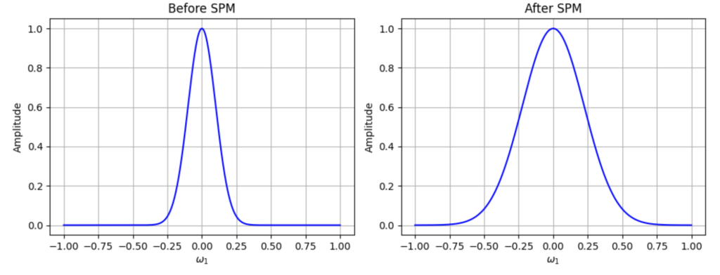
Fig: In SPM, amplitude variations of a signal generate a pattern-dependent nonlinear phase shift on itself, causing spectral broadening and impairing transmission.
-
Spectral Broadening:
- As the pulse propagates, the instantaneous power of the pulse causes a time-dependent phase shift, which in turn results in a frequency chirp. The leading edge of the pulse is red-shifted, while the trailing edge is blue-shifted. This phenomenon leads to broadening of the optical spectrum.
-
Impact on Chromatic Dispersion:
- SPM interacts with chromatic dispersion in the fiber. If the dispersion is anomalous (negative), SPM can counteract dispersion-induced pulse broadening. However, in the normal dispersion regime, SPM enhances pulse broadening, worsening signal degradation.
-
Phase Distortion:
- The nonlinear phase shift introduced by SPM leads to phase distortions, which can degrade the signal’s quality, especially in systems using phase modulation formats like QPSK or QAM.
-
Pulse Distortion:
- The interplay between SPM and fiber dispersion can lead to significant pulse distortion, which limits the maximum transmission distance before signal regeneration or dispersion compensation is required.
SPM in WDM Systems
While SPM primarily affects single-channel systems, it also plays a role in wavelength-division multiplexing (WDM) systems. In WDM systems, SPM can interact with cross-phase modulation (XPM) and four-wave mixing (FWM), leading to inter-channel crosstalk and further performance degradation. In WDM systems, the total nonlinear effect is the combined result of SPM and these inter-channel nonlinear effects.
SPM in Coherent Systems
In coherent optical systems, which use advanced digital signal processing (DSP), the impact of SPM can be mitigated to some extent by using nonlinear compensation techniques. Coherent systems detect both the phase and amplitude of the signal, allowing for more efficient compensation of nonlinear phase distortions. However, SPM still imposes limits on the maximum transmission distance and system capacity.
Mitigation of SPM
Several techniques are employed to reduce the impact of SPM in optical fiber systems:
-
Lowering Launch Power:
- Reducing the optical power launched into the fiber can reduce the nonlinear phase shift caused by SPM. However, this approach must be balanced with maintaining a sufficient signal-to-noise ratio (SNR).
-
Dispersion Management:
- Carefully managing the dispersion in the fiber can help reduce the interplay between SPM and chromatic dispersion. By compensating for dispersion, it is possible to limit pulse broadening and signal degradation.
-
Advanced Modulation Formats:
- Modulation formats that are less sensitive to phase distortions, such as differential phase-shift keying (DPSK), can reduce the impact of SPM on the signal.
-
Digital Signal Processing (DSP):
- In coherent systems, DSP algorithms are used to compensate for the phase distortions caused by SPM. These algorithms reconstruct the original signal by reversing the nonlinear phase shift introduced during propagation.
Practical Applications of SPM
Despite its negative effects on signal quality, SPM can also be exploited for certain beneficial applications:
-
All-Optical Regeneration:
- SPM has been used in all-optical regenerators, where the spectral broadening caused by SPM is filtered to suppress noise and restore signal integrity. By filtering the broadened spectrum, the regenerator can remove low-power noise components while maintaining the data content.
-
Optical Solitons:
- In systems designed to use optical solitons, the effects of SPM and chromatic dispersion are balanced to maintain pulse shape over long distances. Solitons are stable pulses that do not broaden or compress during propagation, making them useful for long-haul communication.
SPM in Submarine Systems
In ultra-long-haul submarine optical systems, where transmission distances can exceed several thousand kilometers, SPM plays a critical role in determining the system’s performance. SPM interacts with chromatic dispersion and other nonlinear effects to limit the achievable transmission distance. To mitigate the effects of SPM, submarine systems often employ advanced nonlinear compensation techniques, including optical phase conjugation and digital back-propagation.
Summary
Self-phase modulation (SPM) is a significant nonlinear effect in optical fiber communication, particularly in high-power, long-distance systems. It leads to spectral broadening and phase distortion, which degrade the signal quality. While SPM can limit the performance of optical systems, it can also be leveraged for applications like all-optical regeneration. Proper management of SPM is essential for achieving high-capacity, long-distance optical transmission, particularly in coherent systems and submarine cable networks.Some of the quick key take-aways are :-
-
-
- In coherent optical networks, SPM (Self-Phase Modulation) occurs when the intensity of the light signal alters its phase, leading to changes in the signal’s frequency spectrum as it travels through the fiber.
- Higher signal power levels make SPM more pronounced in coherent systems, so managing optical power is crucial to maintaining signal quality.
- SPM causes spectral broadening, which can lead to signal overlap and distortion, especially in Dense Wavelength Division Multiplexing (DWDM) systems with closely spaced channels.
- In long-haul coherent networks, fiber length increases the cumulative effect of SPM, making it necessary to incorporate compensation mechanisms to maintain signal integrity.
- Optical amplifiers, such as EDFA and Raman amplifiers, increase signal power, which can trigger SPM effects in coherent systems, requiring careful design and power control.
- Dispersion management is essential in coherent networks to mitigate the interaction between SPM and dispersion, which can further distort the signal. By balancing these effects, signal degradation is reduced.
- In coherent systems, advanced modulation formats like Quadrature Amplitude Modulation (QAM) and coherent detection help improve the system’s resilience to SPM, although higher modulation formats may still be sensitive to nonlinearities.
- Digital signal processing (DSP) is widely used in coherent systems to compensate for the phase distortions introduced by SPM, restoring signal quality after transmission through long fiber spans.
- Nonlinear compensation algorithms in DSP specifically target SPM effects, allowing coherent systems to operate effectively even in the presence of high power and long-distance transmission.
- Channel power optimization and careful spacing in DWDM systems are critical strategies for minimizing the impact of SPM in coherent optical networks, ensuring better performance and higher data rates.
-
Reference
- https://optiwave.com/opti_product/optical-system-spm-induced-spectral-broadening/
 in DWDM Networks")
Polarization Mode Dispersion (PMD) is one of the significant impairments in optical fiber communication systems, particularly in Dense Wavelength Division Multiplexing (DWDM) systems where multiple wavelengths (channels) are transmitted simultaneously over a single optical fiber. PMD occurs because of the difference in propagation velocities between two orthogonal polarization modes in the fiber. This difference results in a broadening of the optical pulses over time, leading to intersymbol interference (ISI), degradation of signal quality, and increased bit error rates (BER).
PMD is caused by imperfections in the optical fiber, such as slight variations in its shape, stress, and environmental factors like temperature changes. These factors cause the fiber to become birefringent, meaning that the refractive index experienced by light depends on its polarization state. As a result, light polarized in one direction travels at a different speed than light polarized in the perpendicular direction.
The Physics of PMD
PMD arises from the birefringence of optical fibers. Birefringence is the difference in refractive index between two orthogonal polarization modes in the fiber, which results in different group velocities for these modes. The difference in arrival times between the two polarization components is called the Differential Group Delay (DGD).
The DGD is given by:
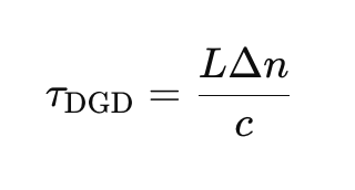
Where:
- L is the length of the fiber.
- Δn is the difference in refractive index between the two polarization modes.
- c is the speed of light in vacuum.
This DGD causes pulse broadening, as different polarization components of the signal arrive at the receiver at different times. Over long distances, this effect can accumulate and become a major impairment in optical communication systems.
Polarization Mode Dispersion and Pulse Broadening
The primary effect of PMD is pulse broadening, which occurs when the polarization components of the optical signal are delayed relative to one another. This leads to intersymbol interference (ISI), as the broadened pulses overlap with adjacent pulses, making it difficult for the receiver to distinguish between symbols. The amount of pulse broadening increases with the DGD and the length of the fiber.
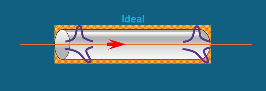
The PMD coefficient is typically measured in ps/√km, which represents the DGD per unit length of fiber. For example, in standard single-mode fibers (SSMF), the PMD coefficient is typically around 0.05–0.5 ps/√km. Over long distances, the total DGD can become significant, leading to substantial pulse broadening.
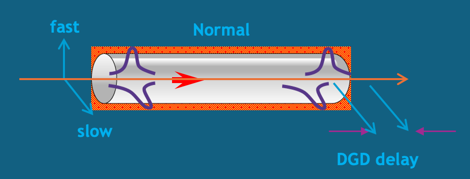
Statistical Nature of PMD
PMD is inherently stochastic, meaning that it changes over time due to environmental factors such as temperature fluctuations, mechanical stress, and fiber bending. These changes cause the birefringence of the fiber to vary randomly, making PMD difficult to predict and compensate for. The random nature of PMD is usually described using statistical models, such as the Maxwellian distribution for DGD.
The mean DGD increases with the square root of the fiber length, as given by:
Where:
- τPMD is the PMD coefficient of the fiber.
- L is the length of the fiber.
PMD in Coherent Systems
In modern coherent optical communication systems, PMD can have a severe impact on system performance. Coherent systems rely on both the phase and amplitude of the received signal to recover the transmitted data, and any phase distortions caused by PMD can lead to significant degradation in signal quality. PMD-induced phase shifts lead to phase noise, which in turn increases the bit error rate (BER).
Systems using advanced modulation formats, such as Quadrature Amplitude Modulation (QAM), are particularly sensitive to PMD, as these formats rely on accurate phase information to recover the transmitted data. The nonlinear phase noise introduced by PMD can interfere with the receiver’s ability to correctly demodulate the signal, leading to increased errors.
Formula for PMD-Induced Pulse Broadening
The pulse broadening due to PMD can be expressed as:
Where:
- τDGD is the differential group delay.
- L is the fiber length.
This equation shows that the amount of pulse broadening increases with both the DGD and the fiber length. Over long distances, the cumulative effect of PMD can cause significant ISI and degrade system performance.
Detecting PMD in DWDM Systems
Engineers can detect PMD in DWDM networks by monitoring several key performance indicators (KPIs):
- Increased Bit Error Rate (BER): PMD-induced phase noise and pulse broadening lead to higher BER, particularly in systems using high-speed modulation formats like QAM.
-
-
-
-
- KPI: Real-time BER monitoring. A significant increase in BER, especially over long distances, is a sign of PMD.
-
-
-
-
- Signal-to-Noise Ratio (SNR) Degradation: PMD introduces phase noise and pulse broadening, which degrade the SNR. Operators may observe a drop in SNR in the affected channels.
-
-
-
-
- KPI: SNR monitoring tools that provide real-time feedback on the quality of the transmitted signal.
-
-
-
-
- Pulse Shape Distortion: PMD causes temporal pulse broadening and distortion. Using an optical sampling oscilloscope, operators can visually inspect the shape of the transmitted pulses to identify any broadening caused by PMD.
- Optical Spectrum Analyzer (OSA): PMD can lead to spectral broadening of the signal, which can be detected using an OSA. The analyzer will show the broadening of the spectrum of the affected channels, indicating the presence of PMD.
Mitigating PMD in DWDM Systems
Several strategies can be employed to mitigate the effects of PMD in DWDM systems:
- PMD Compensation Modules: These are adaptive optical devices that compensate for the differential group delay introduced by PMD. They can be inserted periodically along the fiber link to reduce the total accumulated PMD.
- Digital Signal Processing (DSP): In modern coherent systems, DSP techniques can be used to compensate for the effects of PMD at the receiver. These methods involve applying adaptive equalization filters to reverse the effects of PMD.
- Fiber Design: Fibers with lower PMD coefficients can be used to reduce the impact of PMD. Modern optical fibers are designed to minimize birefringence and reduce the amount of PMD.
- Polarization Multiplexing: In polarization multiplexing systems, PMD can be mitigated by separating the signals transmitted on orthogonal polarization states and applying adaptive equalization to each polarization component.
- Advanced Modulation Formats: Modulation formats that are less sensitive to phase noise, such as Differential Phase-Shift Keying (DPSK), can help reduce the impact of PMD on system performance.
Polarization Mode Dispersion (PMD) is a critical impairment in DWDM networks, causing pulse broadening, phase noise, and intersymbol interference. It is inherently stochastic, meaning that it changes over time due to environmental factors, making it difficult to predict and compensate for. However, with the advent of digital coherent optical systems and DSP techniques, PMD can be effectively managed and compensated for, allowing modern systems to achieve high data rates and long transmission distances without significant performance degradation.
Summary
- Different polarization states of light travel at slightly different speeds in a fiber, causing pulse distortion.
- This variation can cause pulses to overlap or alter their shape enough to become undetectable at the receiver.
- PMD occurs when the main polarization mode travels faster than the secondary mode, causing a delay known as Differential Group Delay (DGD).
- PMD becomes problematic at higher transmission rates like 10, 40 or 100 Gbps etc.
- Unlike chromatic dispersion, PMD is a statistical, non-linear phenomenon, making it more complex to manage.
- PMD is caused by fiber asymmetry due to geometric imperfections, stress from the wrapping material, manufacturing processes, or mechanical stress during cable laying.
- PMD is the average value of DGD distributions, which vary over time, and thus cannot be directly measured in the field.
Reference
- https://www.wiley.com/en-ie/Fiber-Optic+Communication+Systems%2C+5th+Edition-p-9781119737360
 in DWDM Networks")
Chromatic Dispersion (CD) is a key impairment in optical fiber communication, especially in Dense Wavelength Division Multiplexing (DWDM) systems. It occurs due to the variation of the refractive index of the optical fiber with the wavelength of the transmitted light. Since different wavelengths travel at different speeds through the fiber, pulses of light that contain multiple wavelengths spread out over time, leading to pulse broadening. This broadening can cause intersymbol interference (ISI), degrading the signal quality and ultimately increasing the bit error rate (BER) in the network.With below details,I believe reader will be able to understand all about CD in the DWDM system.I have added some figures which can help visualise the affect of CD.
Physics behind Chromatic Dispersion
CD results from the fact that optical fibers have both material dispersion and waveguide dispersion. The material dispersion arises from the inherent properties of the silica material, while waveguide dispersion results from the interaction between the core and cladding of the fiber. These two effects combine to create a wavelength-dependent group velocity, causing different spectral components of an optical signal to travel at different speeds.
The relationship between the group velocity Vg and the propagation constant β is given by:
 where:
- ω is the angular frequency.
- β is the propagation constant.
The propagation constant β typically varies nonlinearly with frequency in optical fibers. This nonlinear dependence is what causes different frequency components to propagate with different group velocities, leading to CD.
Chromatic Dispersion Effects in DWDM Systems
In DWDM systems, where multiple closely spaced wavelengths are transmitted simultaneously, chromatic dispersion can cause significant pulse broadening. Over long fiber spans, this effect can spread the pulses enough to cause overlap between adjacent symbols, leading to ISI. The severity of CD increases with:
- Fiber length: The longer the fiber, the more time the different wavelength components have to disperse.
- Signal bandwidth: A broader signal (wider range of wavelengths) is more susceptible to dispersion.
The amount of pulse broadening due to CD can be quantified by the Group Velocity Dispersion (GVD) parameter D, typically measured in ps/nm/km. The GVD represents the time delay per unit wavelength shift, per unit length of the fiber. The relation between the GVD parameter D and the second-order propagation constant β2 is:
Where:
- c is the speed of light in vacuum.
- λ is the operating wavelength.
Pulse Broadening Due to CD
The pulse broadening (or time spread) due to CD is given by:
 Where:
- D is the GVD parameter.
- L is the length of the fiber.
- Δλ is the spectral bandwidth of the signal.
For example, in a standard single-mode fiber (SSMF) with D=17 ps/nm/km at a wavelength of 1550 nm, a signal with a spectral width of 0.4 nm transmitted over 1000 km will experience significant pulse broadening, potentially leading to ISI and performance degradation in the network.
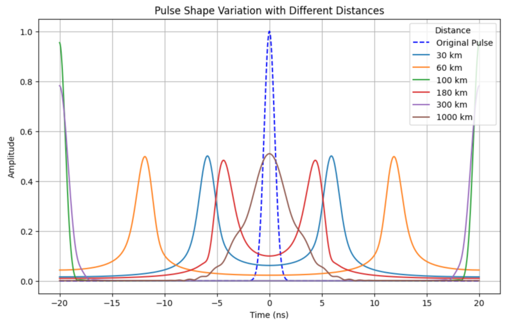
CD in Coherent Systems
In modern coherent optical systems, CD can be compensated for using digital signal processing (DSP) techniques. At the receiver, the distorted signal is passed through adaptive equalizers that reverse the effects of CD. This approach allows for complete digital compensation of chromatic dispersion, making it unnecessary to use optical dispersion compensating modules (DCMs) that were commonly used in older systems.
Chromatic Dispersion Profiles in Fibers
CD varies with wavelength. For standard single-mode fibers (SSMFs), the CD is positive and increases with wavelength beyond 1300 nm. DSFs were developed to shift the zero-dispersion wavelength from 1300 nm to 1550 nm, where fiber attenuation is minimized, making them suitable for older single-channel systems. However, in modern DWDM systems, DSFs are less preferred due to their smaller core area, which enhances nonlinear effects at high power levels .
Link to see CD in action
Impact of CD on System Performance
- Intersymbol Interference (ISI): As CD broadens the pulses, they start to overlap, causing ISI. This effect increases the BER, particularly in systems with high symbol rates and wide bandwidths.
- Signal-to-Noise Ratio (SNR) Degradation: CD can reduce the effective SNR by spreading the signal over a wider temporal window, making it harder for the receiver to recover the original signal.
- Spectral Efficiency: CD limits the maximum data rate that can be transmitted over a given bandwidth, reducing the spectral efficiency of the system.
- Increased Bit Error Rate (BER): The ISI caused by CD can lead to higher BER, particularly over long distances or at high data rates. The degradation becomes more pronounced at higher bit rates because the pulses are narrower, and thus more susceptible to dispersion.
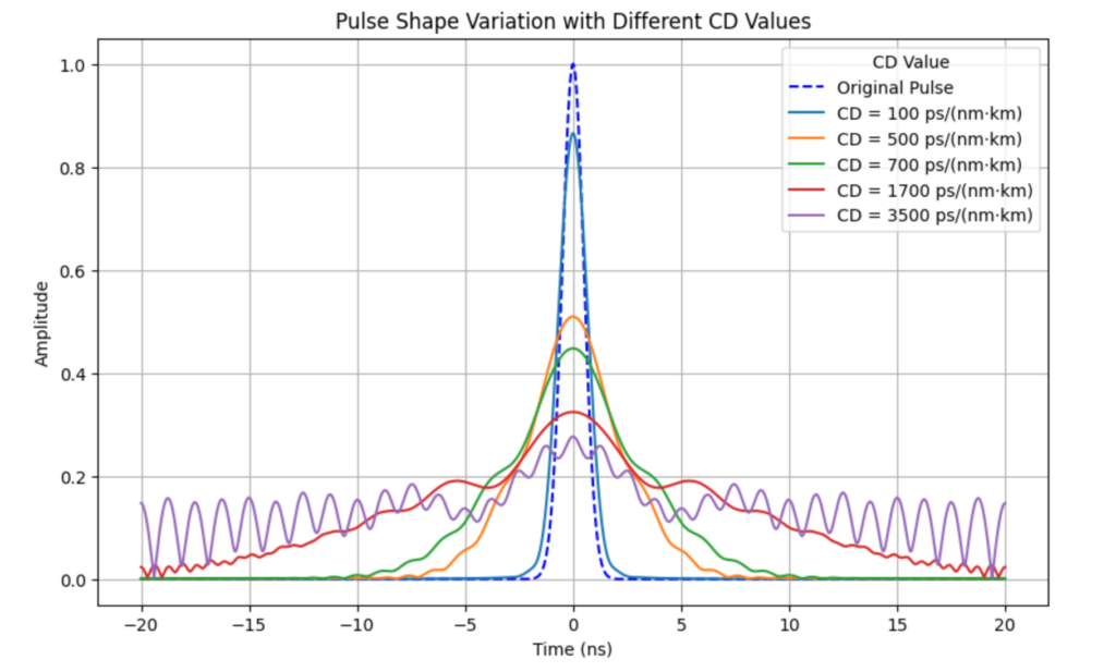
Detection of CD in DWDM Systems
Operators can detect the presence of CD in DWDM networks by monitoring several key indicators:
- Increased BER: The first sign of CD is usually an increase in the BER, particularly in systems operating at high data rates. This increase occurs due to the intersymbol interference caused by pulse broadening.
- Signal-to-Noise Ratio (SNR) Degradation: CD can reduce the SNR, which can be observed using real-time monitoring tools.
- Pulse Shape Distortion: CD causes temporal pulse broadening and distortion. Using an optical sampling oscilloscope, operators can visually inspect the shape of the transmitted pulses to identify any broadening caused by CD.
- Optical Spectrum Analyzer (OSA): An OSA can be used to detect the broadening of the signal’s spectrum, which is a direct consequence of chromatic dispersion.
Mitigating Chromatic Dispersion
There are several strategies for mitigating CD in DWDM networks:
- Dispersion Compensation Modules (DCMs): These are optical devices that introduce negative dispersion to counteract the positive dispersion introduced by the fiber. DCMs can be placed periodically along the link to reduce the total accumulated dispersion.
- Digital Signal Processing (DSP): In modern coherent systems, CD can be compensated for using DSP techniques at the receiver. These methods involve applying adaptive equalization filters to reverse the effects of dispersion.
- Dispersion-Shifted Fibers (DSFs): These fibers are designed to shift the zero-dispersion wavelength to minimize the effects of CD. However, they are less common in modern systems due to the increase in nonlinear effects.
- Advanced Modulation Formats: Modulation formats that are less sensitive to ISI, such as Differential Phase-Shift Keying (DPSK), can help reduce the impact of CD on system performance.
Chromatic Dispersion (CD) is a major impairment in optical communication systems, particularly in long-haul DWDM networks. It causes pulse broadening and intersymbol interference, which degrade signal quality and increase the bit error rate. However, with the availability of digital coherent optical systems and DSP techniques, CD can be effectively managed and compensated for, allowing modern systems to achieve high data rates and long transmission distances without significant performance degradation.
Reference
https://webdemo.inue.uni-stuttgart.de/

In modern optical fiber communications, maximizing data transmission efficiency while minimizing signal degradation is crucial. Several key parameters such as baud rate, bit rate, and spectral width play a critical role in determining the performance of optical networks. I have seen we discuss these parameters so many time during our technical discussion and still there is lot of confusion, so I thought of compiling all the information which is available in bits and pieces.This article will deep dive into all these concepts, their dependencies, and how modulation schemes influence their behavior in optical systems.
Baud Rate vs. Bit Rate
At the core of digital communication, the bit rate represents the amount of data transmitted per second, measured in bits per second (bps). The baud rate, on the other hand, refers to the number of symbol changes or signaling events per second, measured in symbols per second (baud). While these terms are often used interchangeably, they describe different aspects of signal transmission.In systems with simple modulation schemes, such as Binary Phase Shift Keying (BPSK), where one bit is transmitted per symbol, the baud rate equals the bit rate. However, as more advanced modulation schemes are introduced (e.g., Quadrature Amplitude Modulation or QAM), multiple bits can be encoded in each symbol, leading to situations where the bit rate exceeds the baud rate. The relationship between baud rate, bit rate, and the modulation order (number of bits per symbol) is given by:
Where:
- B = Bit rate (bps)
- S = Baud rate (baud)
- m = Modulation order (number of symbols)
The baud rate represents the number of symbols transmitted per second, while the bit rate is the total number of bits transmitted per second. Engineers often need to choose an optimal balance between baud rate and modulation format based on the system’s performance requirements. For example:
- High baud rates can increase throughput, but they also increase the spectral width and require more sophisticated filtering and higher-quality optical components.
- Higher-order modulation formats (e.g., 16-QAM, 64-QAM) allow engineers to increase the bit rate without expanding the spectral width. However, these modulation formats require a higher Signal-to-Noise Ratio (SNR) to maintain acceptable Bit Error Rates (BER).
Choosing the right baud rate and modulation format depends on factors such as available bandwidth, distance, and power efficiency. For example, in a long-haul optical system, engineers may opt for lower-order modulation (like QPSK) to maintain signal integrity over vast distances, while in shorter metro links, higher-order modulation (like 16-QAM or 64-QAM) might be preferred to maximize data throughput.
Spectral Width
The spectral width of a signal defines the range of frequencies required for transmission. In the context of coherent optical communications, spectral width is directly related to the baud rate and the roll-off factor used in filtering. It can be represented by the formula:
Spectral Width=Baud Rate×(1+Roll-off Factor)
The spectral width of an optical signal determines the amount of frequency spectrum it occupies, which directly affects how efficiently the system uses bandwidth. The roll-off factor (α) in filters impacts the spectral width:
- Lower roll-off factors reduce the bandwidth required but make the signal more susceptible to inter-symbol interference (ISI).
- Higher roll-off factors increase the bandwidth but offer smoother transitions between symbols, thus reducing ISI.
In systems where bandwidth is a critical resource such as Dense Wavelength Division Multiplexing (DWDM), engineers need to optimize the roll-off factor to balance spectral efficiency and signal integrity. For example, in a DWDM system with closely spaced channels, a roll-off factor of 0.1 to 0.2 is typically used to avoid excessive inter-channel crosstalk.
For example, if a signal is transmitted at a baud rate of 64 GBaud with a roll-off factor of 0.2, the actual bandwidth required for transmission becomes:
Bandwidth=64×(1+0.2)=76.8GHz
This relationship is crucial in Dense Wavelength Division Multiplexing (DWDM) systems, where spectral width must be tightly controlled to avoid interference between adjacent channels.
The Nyquist Theorem and Roll-Off Factor
The Nyquist theorem sets a theoretical limit on the minimum bandwidth required to transmit data without ISI. According to this theorem, the minimum bandwidth Bmin for a signal is half the baud rate:
 In practical systems, the actual bandwidth exceeds this minimum due to imperfections in filters and other system limitations. The roll-off factor r typically ranging from 0 to 1, defines the excess bandwidth required beyond the Nyquist limit. The actual bandwidth with a roll-off factor is:
Bactual=Baud Rate×(1+r)
Choosing an appropriate roll-off factor involves balancing bandwidth efficiency with system robustness. A higher roll-off factor results in smoother transitions between symbols and reduced ISI but at the cost of increased bandwidth consumption.
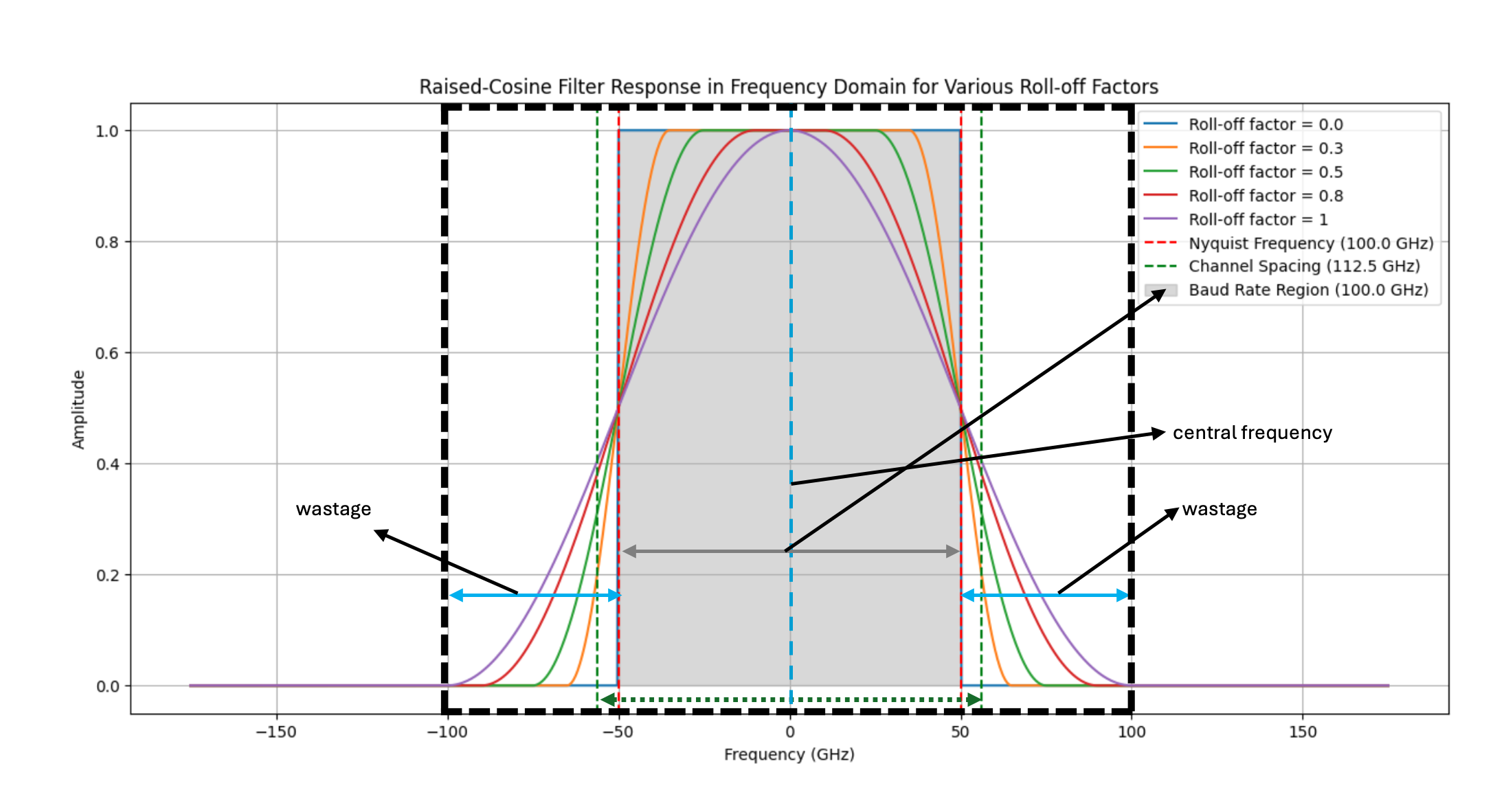
Fig: Raised-cosine filter response showing the effect of various roll-off factors on bandwidth efficiency. Highlighted are the central frequency, Nyquist bandwidth, and wasted spectral bandwidth due to roll-off.
Spectral Efficiency and Channel Bandwidth
The spectral efficiency of an optical communication system, measured in bits per second per Hertz, depends on both the baud rate and the modulation scheme. It can be expressed as:
For modern coherent optical systems, achieving high spectral efficiency is crucial for maximizing the data capacity of fiber-optic channels, especially in DWDM systems where multiple channels are transmitted over the same fiber.
Calculation of Bit Rate and Spectral Efficiency
Consider a 50 Gbaud system using 16-QAM modulation. The bit rate can be calculated as follows:
Bit Rate=50 Gbaud×4 bits/symbol=200 Gbps
Assuming a roll-off factor α=0.2 , the spectral width would be:
![]()
Thus, the spectral efficiency is:
This example demonstrates how increasing the modulation order (in this case, 16-QAM) boosts the bit rate, while maintaining acceptable spectral efficiency.
Trade-offs Between Baud Rate, Bit Rate and Modulation Formats
In optical communication systems, higher baud rates allow for the transmission of more symbols per second, but they require broader spectral widths (i.e., more bandwidth). Conversely, higher-order modulation formats allow more bits per symbol, reducing the required baud rate for the same bit rate, but they increase system complexity and susceptibility to impairments.
For instance, if we aim to transmit a 400 Gbps signal, we have two general options:
- Increasing the Baud Rate: Keeping a lower modulation format (e.g., QPSK), we can increase the baud rate. For instance, a 400 Gbps signal using QPSK requires a 200 GBaud rate.
- Using Higher-Order Modulation: With 64-QAM, which transmits 6 bits per symbol, we could transmit the same 400 Gbps with a baud rate of approximately 66.67 GBaud.
While higher baud rates increase the spectral width requirement, they are generally less sensitive to noise. Higher-order modulation schemes, on the other hand, require less spectral width but need a higher optical signal-to-noise ratio (OSNR) to maintain performance. Engineers need to carefully balance baud rate and modulation formats based on system requirements and constraints.
Practical Applications of Baud Rate and Modulation Schemes in Real-World Networks
High-speed optical communication systems rely heavily on factors such as baud rate, bit rate, spectral width, and roll-off factor to optimize performance. Engineers working with fiber-optic systems continuously face the challenge of optimizing these parameters to achieve maximum signal reach, data capacity, and power efficiency. To overcome the physical limitations of optical fibers and system components, Digital Signal Processing (DSP) plays a pivotal role in enabling high-capacity data transmission while minimizing signal degradation. This extended article dives deeper into the real-world applications of these concepts and how engineers modify and optimize DSP to improve system performance.
When Do Engineers Need This Information?
Optical engineers need to understand the relationships between baud rate, spectral width, bit rate, and DSP when designing and maintaining high-speed communication networks, especially for:
- Long-haul fiber-optic systems (e.g., transoceanic communication lines),
- Metro networks where high data rates are required over moderate distances,
- Data center interconnects that demand ultra-low latency and high throughput,
- 5G backhaul networks, where efficient use of bandwidth and high data rates are essential.
How Engineers Use DSP to Optimize Signal Performance?
Pre-Equalization for Baud Rate and Bandwidth Optimization
In optical systems with high baud rates (e.g., 64 Gbaud and above), the signal may be degraded due to limited bandwidth in the optical components, such as transmitters and amplifiers. Engineers use pre-equalization techniques in the DSP to pre-compensate for these bandwidth limitations. By shaping the signal before transmission, pre-equalization ensures that the signal maintains its integrity throughout the transmission process.
For instance, a 100 Gbaud signal may suffer from component bandwidth limitations, resulting in signal distortion. Engineers can use DSP to pre-distort the signal, allowing it to pass through the limited-bandwidth components without significant degradation.
Adaptive Equalization for Signal Reach Optimization
To maximize the reach of optical signals, engineers use adaptive equalization algorithms, which dynamically adjust the signal to compensate for impairments encountered during transmission. One common algorithm is the decision-directed least mean square (DD-LMS) equalizer, which adapts the system’s response to continuously minimize errors in the received signal.This is particularly important in long-haul and submarine optical networks, where signals travel thousands of kilometers and are subject to various impairments such as chromatic dispersion and fiber nonlinearity.
Polarization Mode Dispersion (PMD) Compensation
In optical systems, polarization mode dispersion (PMD) causes signal distortion by splitting light into two polarization modes that travel at different speeds. DSP is used to track and compensate for PMD in real-time, ensuring that the signal arrives at the receiver without significant polarization-induced distortion.
Practical Example of DSP Optimization in Super-Nyquist WDM Systems
In super-Nyquist WDM systems, where the channel spacing is narrower than the baud rate, DSP plays a crucial role in ensuring spectral efficiency while maintaining signal integrity. By employing advanced multi-modulus blind equalization algorithms, engineers can effectively mitigate inter-channel interference (ICI) and ISI. This allows the system to transmit data at rates higher than the Nyquist limit, thereby improving spectral efficiency.
For example, consider a super-Nyquist system transmitting 400 Gbps signals with a 50 GHz channel spacing. In this case, the baud rate exceeds the available bandwidth, leading to spectral overlap. DSP compensates for the resulting crosstalk and ISI, enabling the system to achieve high spectral efficiency (e.g., 4 bits/s/Hz) while maintaining a low BER.
How Roll-Off Factor Affects Spectral Width and Signal Reach
The roll-off factor directly affects the bandwidth used by a signal. In systems where spectral efficiency is critical (such as DWDM networks), engineers may opt for a lower roll-off factor (e.g., 0.1 to 0.2) to reduce the bandwidth and fit more channels into the same optical spectrum. However, this requires more sophisticated DSP algorithms to manage the increased ISI that results from narrower filters.
For example, in a DWDM system operating at 50 GHz channel spacing, a low roll-off factor allows for tighter channel packing but necessitates more advanced ISI compensation through DSP. Conversely, a higher roll-off factor reduces the need for ISI compensation but increases the required bandwidth, limiting the number of channels that can be transmitted.
The Role of DSP in Power Optimization
Power efficiency is another crucial consideration in optical systems, especially in long-haul and submarine networks where power consumption can significantly impact operational costs. DSP allows engineers to optimize power by:
- Pre-distorting the signal to reduce the impact of non-linearities, enabling the use of lower transmission power while maintaining signal quality.
- Compensating for impairments such as self-phase modulation (SPM) and cross-phase modulation (XPM), which are power-dependent effects that degrade signal quality.
By using DSP to manage power-efficient transmission, engineers can extend the signal reach and reduce the power consumption of optical amplifiers, thereby improving the overall system performance.
References
: A Game-Changer for Optical Communication")
The world of optical communication is undergoing a transformation with the introduction of Hollow Core Fiber (HCF) technology. This revolutionary technology offers an alternative to traditional Single Mode Fiber (SMF) and presents exciting new possibilities for improving data transmission, reducing costs, and enhancing overall performance. In this article, we will explore the benefits, challenges, and applications of HCF, providing a clear and concise guide for optical fiber engineers.

What is Hollow Core Fiber (HCF)?
Hollow Core Fiber (HCF) is a type of optical fiber where the core, typically made of air or gas, allows light to pass through with minimal interference from the fiber material. This is different from Single Mode Fiber (SMF), where the core is made of solid silica, which can introduce problems like signal loss, dispersion, and nonlinearities.
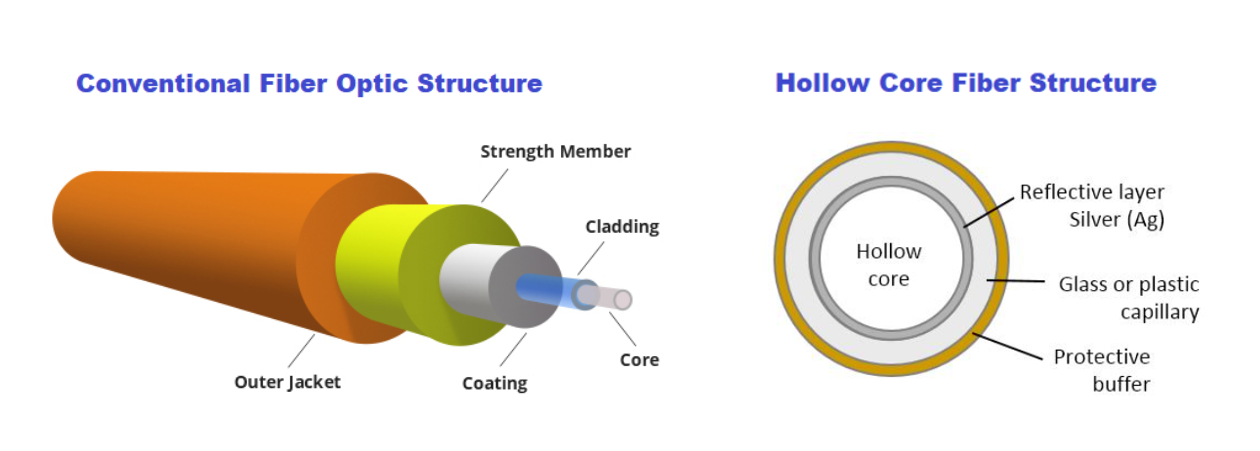
In HCF, light travels through the hollow core rather than being confined within a solid medium. This design offers several key advantages that make it an exciting alternative for modern communication networks.
Traditional SMF vs. Hollow Core Fiber (HCF)
Single Mode Fiber (SMF) technology has dominated optical communication for decades. Its core is made of silica, which confines laser light, but this comes at a cost in terms of:
- Attenuation: SMF exhibits more than 0.15 dB/km attenuation, necessitating Erbium-Doped Fiber Amplifiers (EDFA) or Raman amplifiers to extend transmission distances. However, these amplifiers add Amplified Spontaneous Emission (ASE) noise, degrading the Optical Signal-to-Noise Ratio (OSNR) and increasing both cost and power consumption.
- Dispersion: SMF suffers from chromatic dispersion (CD), requiring expensive Dispersion Compensation Fibers (DCF) or power-hungry Digital Signal Processing (DSP) for compensation. This increases the size of the transceiver (XCVR) and overall system costs.
- Nonlinearity: SMF’s inherent nonlinearities limit transmission power and distance, which affects overall capacity. Compensation for these nonlinearities, usually handled at the DSP level, increases the system’s complexity and power consumption.
- Stimulated Raman Scattering (SRS): This restricts wideband transmission and requires compensation mechanisms at the amplifier level, further increasing cost and system complexity.
In contrast, Hollow Core Fiber (HCF) offers significant advantages:
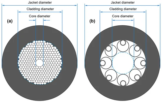
- Attenuation: Advanced HCF types, such as Nested Anti-Resonant Nodeless Fiber (NANF), achieve attenuation rates below 0.1 dB/km, especially in the O-band, matching the performance of the best SMF in the C-band.
- Low Dispersion and Nonlinearity: HCF exhibits almost zero CD and nonlinearity, which eliminates the need for complex DSP systems and increases the system’s capacity for higher-order modulation schemes over long distances.
- Latency: The hollow core reduces latency by approximately 33%, making it highly attractive for latency-sensitive applications like high-frequency trading and satellite communications.
- Wideband Transmission: With minimal SRS, HCF allows ultra-wideband transmission across O, E, S, C, L, and U bands, making it ideal for next-generation optical systems.
Operational Challenges in Deploying HCF
Despite its impressive benefits, HCF also presents some challenges that engineers need to address when deploying this technology.
1. Splicing and Connector Challenges
Special care must be taken when connecting HCF cables. The hollow core can allow air to enter during splicing or through connectors, which increases signal loss and introduces nonlinear effects. Special connectors are required to prevent air ingress, and splicing between HCF and SMF needs careful alignment to avoid high losses. Fortunately, methods like thermally expanded core (TEC) technology have been developed to improve the efficiency of these connections.
2. Amplification Issues
Amplifying signals in HCF systems can be challenging due to air-glass reflections at the interfaces between different fiber types. Special isolators and mode field couplers are needed to ensure smooth amplification without signal loss.
3. Bend Sensitivity
HCF fibers are more sensitive to bending than traditional SMF. While this issue is being addressed with new designs, such as Photonic Crystal Fibers (PCF), engineers still need to handle HCF with care during installation.
4. Fault Management
HCF has a lower back reflection compared to SMF, which makes it harder to detect faults using traditional Optical Time Domain Reflectometry (OTDR). New low-cost OTDR systems are being developed to overcome this issue, offering better fault detection in HCF systems.

(a) Schematics of a 3×4-slot mating sleeve and two CTF connectors; (b) principle of lateral offset reduction by using a multi-slot mating sleeve; (c) Measured ILs (at 1550 nm) of a CTF/CTF interconnection versus the relative rotation angle; (d) Minimum ILs of 10 plugging trials.
Applications of Hollow Core Fiber
HCF is already being used in several high-demand applications, and its potential continues to grow.
1. Financial Trading Networks
HCF’s low-latency properties make it ideal for high-frequency trading (HFT) systems, where reducing transmission delay can provide a competitive edge. The London Stock Exchange has implemented HCF to speed up transactions, and this use case is expanding across financial hubs globally.
2. Data Centers
The increasing demand for fast, high-capacity data transfer in data centers makes HCF an attractive solution. Anti-resonant HCF designs are being tested for 800G applications, which significantly reduce the need for frequent signal amplification, lowering both cost and energy consumption.
3. Submarine Communication Systems
Submarine cables, which carry the majority of international internet traffic, benefit from HCF’s low attenuation and high power transmission capabilities. HCF can transmit kilowatt-level power over long distances, making it more efficient than traditional fiber in submarine communication networks.
4. 5G Networks and Remote Radio Access
As 5G networks expand, Remote Radio Units (RRUs) are increasingly connected to central offices through HCF. HCF’s ability to cover larger geographic areas with low latency helps 5G providers increase their coverage while reducing costs. This technology also allows networks to remain resilient, even during outages, by quickly switching between units.
Future Directions for HCF Technology
HCF is poised to shift the focus of optical transmission from the C-band to the O-band, thanks to its ability to maintain low chromatic dispersion and attenuation in this frequency range. This shift could reduce costs for long-distance communication by simplifying the required amplification and signal processing systems.
In addition, research into high-power transmission through HCF is opening up new opportunities for applications that require the delivery of kilowatts of power over several kilometers. This is especially important for data centers and other critical infrastructures that need reliable power transmission to operate smoothly during grid failures.
Hollow Core Fiber (HCF) represents a leap forward in optical communication technology. With its ability to reduce latency, minimize signal loss, and support high-capacity transmission over long distances, HCF is set to revolutionize industries from financial trading to data centers and submarine networks.
While challenges such as splicing, amplification, and bend sensitivity remain, the ongoing development of new tools and techniques is making HCF more accessible and affordable. For optical fiber engineers, understanding and mastering this technology will be key to designing the next generation of communication networks.
As HCF technology continues to advance, it offers exciting potential for building faster, more efficient, and more reliable optical networks that meet the growing demands of our connected world.
References/Credit :
- Image https://www.holightoptic.com/what-is-hollow-core-fiber-hcf%EF%BC%9F/
- https://www.mdpi.com/2076-3417/13/19/10699
- https://opg.optica.org/oe/fulltext.cfm?uri=oe-30-9-15149&id=471571
- https://www.ofsoptics.com/a-hollow-core-fiber-cable-for-low-latency-transmission-when-microseconds-count/

Introduction
A Digital Twin Network (DTN) represents a major innovation in networking technology, creating a virtual replica of a physical network. This advanced technology enables real-time monitoring, diagnosis, and control of physical networks by providing an interactive mapping between the physical and digital domains. The concept has been widely adopted in various industries, including aerospace, manufacturing, and smart cities, and is now being explored to meet the growing complexities of telecommunication networks.
Here we will deep dive into the fundamentals of Digital Twin Networks, their key requirements, architecture, and security considerations, based on the ITU-T Y.3090 Recommendation.
What is a Digital Twin Network?
A DTN is a virtual model that mirrors the physical network’s operational status, behavior, and architecture. It enables a real-time interactive relationship between the two domains, which helps in analysis, simulation, and management of the physical network. The DTN leverages technologies such as big data, machine learning (ML), artificial intelligence (AI), and cloud computing to enhance the functionality and predictability of networks.
Key Characteristics of Digital Twin Networks
According to ITU-T Y.3090, a DTN is built upon four core characteristics: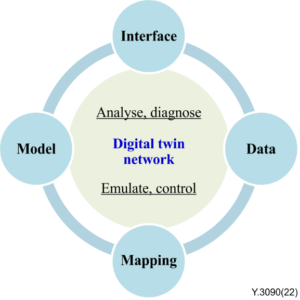
- Data: Data is the foundation of the DTN system. The physical network’s data is stored in a unified digital repository, providing a single source of truth for network applications.
- Real-time Interactive Mapping: The ability to provide a real-time, bi-directional interactive relationship between the physical network and the DTN sets DTNs apart from traditional network simulations.
- Modeling: The DTN contains data models representing various components and behaviors of the network, allowing for flexible simulations and predictions based on real-world data.
- Standardized Interfaces: Interfaces, both southbound (connecting the physical network to the DTN) and northbound (exchanging data between the DTN and network applications), are critical for ensuring scalability and compatibility.
Functional Requirements of DTN
For a DTN to function efficiently, several critical functional requirements must be met:
Efficient Data Collection:
-
-
-
-
-
- The DTN must support massive data collection from network infrastructure, such as physical or logical devices, network topologies, ports, and logs.
- Data collection methods must be lightweight and efficient to avoid strain on network resources.
-
-
-
-
Unified Data Repository:
The data collected is stored in a unified repository that allows real-time access and management of operational data. This repository must support efficient storage techniques, data compression, and backup mechanisms.
Unified Data Models:
-
-
-
-
-
-
-
- The DTN requires accurate and real-time models of network elements, including routers, firewalls, and network topologies. These models allow for real-time simulation, diagnosis, and optimization of network performance.
-
-
-
-
-
-
Open and Standard Interfaces:
-
-
-
-
-
-
-
- Southbound and northbound interfaces must support open standards to ensure interoperability and avoid vendor lock-in. These interfaces are crucial for exchanging information between the physical and digital domains.
-
-
-
-
-
-
Management:
-
-
-
-
-
-
-
- The DTN management function includes lifecycle management of data, topology, and models. This ensures efficient operation and adaptability to network changes.
-
-
-
-
-
-
Service Requirements
Beyond its functional capabilities, a DTN must meet several service requirements to provide reliable and scalable network solutions:
- Compatibility: The DTN must be compatible with various network elements and topologies from multiple vendors, ensuring that it can support diverse physical and virtual network environments.
- Scalability: The DTN should scale in tandem with network expansion, supporting both large-scale and small-scale networks. This includes handling an increasing volume of data, network elements, and changes without performance degradation.
- Reliability: The system must ensure stable and accurate data modeling, interactive feedback, and high availability (99.99% uptime). Backup mechanisms and disaster recovery plans are essential to maintain network stability.
- Security: A DTN must secure sensitive data, protect against cyberattacks, and ensure privacy compliance throughout the lifecycle of the network’s operations.
- Visualization and Synchronization: The DTN must provide user-friendly visualization of network topology, elements, and operations. It should also synchronize with the physical network, providing real-time data accuracy.
Architecture of a Digital Twin Network
The architecture of a DTN is designed to bridge the gap between physical networks and virtual representations. ITU-T Y.3090 proposes a “Three-layer, Three-domain, Double Closed-loop” architecture:
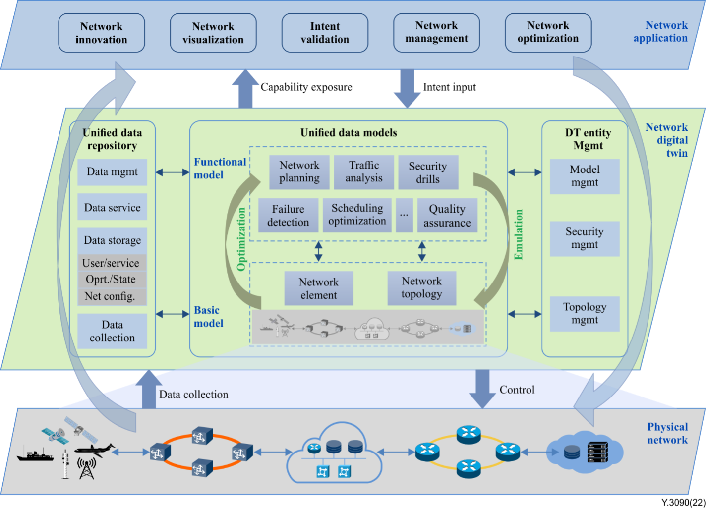
-
Three-layer Structure:
-
-
-
-
- Physical Network Layer: The bottom layer consists of all the physical network elements that provide data to the DTN via southbound interfaces.
- Digital Twin Layer: The middle layer acts as the core of the DTN system, containing subsystems like the unified data repository and digital twin entity management.
- Application Layer: The top layer is where network applications interact with the DTN through northbound interfaces, enabling automated network operations, predictive maintenance, and optimization.
-
-
-
-
-
Three-domain Structure:
-
-
-
-
-
- Data Domain: Collects, stores, and manages network data.
- Model Domain: Contains the data models for network analysis, prediction, and optimization.
- Management Domain: Manages the lifecycle and topology of the digital twin entities.
-
-
-
-
-
-
Double Closed-loop:
-
-
-
-
-
- Inner Loop: The virtual network model is constantly optimized using AI/ML techniques to simulate changes.
- Outer Loop: The optimized solutions are applied to the physical network in real-time, creating a continuous feedback loop between the DTN and the physical network.
-
-
-
-
-
Use Cases of Digital Twin Networks
DTNs offer numerous use cases across various industries and network types:
- Network Operation and Maintenance: DTNs allow network operators to perform predictive maintenance by diagnosing and forecasting network issues before they impact the physical network.
- Network Optimization: DTNs provide a safe environment for testing and optimizing network configurations without affecting the physical network, reducing operating expenses (OPEX).
- Network Innovation: By simulating new network technologies and protocols in the virtual twin, DTNs reduce the risks and costs of deploying innovative solutions in real-world networks.
- Intent-based Networking (IBN): DTNs enable intent-based networking by simulating the effects of network changes based on high-level user intents.
Conclusion
A Digital Twin Network is a transformative concept that will redefine how networks are managed, optimized, and maintained. By providing a real-time, interactive mapping between physical and virtual networks, DTNs offer unprecedented capabilities in predictive maintenance, network optimization, and innovation.
As the complexities of networks grow, adopting a DTN architecture will be crucial for ensuring efficient, secure, and scalable network operations in the future.
Reference

In optical fiber communications, a common assumption is that increasing the signal power will enhance performance. However, this isn’t always the case due to the phenomenon of non-linearity in optical fibers. Non-linear effects can degrade signal quality and cause unexpected issues, especially as power levels rise.
Non-Linearity in Optical Fibers
Non-linearity occurs when the optical power in a fiber becomes high enough that the fiber’s properties start to change in response to the light passing through it. This change is mainly due to the interaction between the light waves and the fiber material, leading to the generation of new frequencies and potential signal distortion.
Harmonics and Four-Wave Mixing
One of the primary non-linear effects is the creation of harmonics—new optical frequencies that weren’t present in the original signal. This happens through a process called Four-Wave Mixing (FWM). In FWM, different light wavelengths (λ) interact with each other inside the fiber, producing new wavelengths.
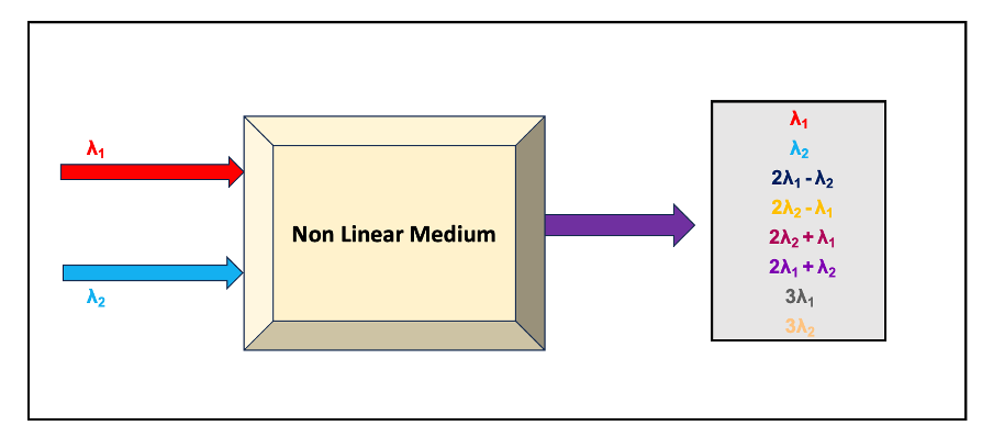


The relationship between these wavelengths can be mathematically described as:
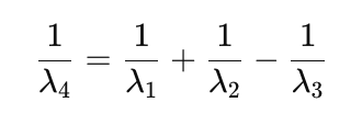 or
or 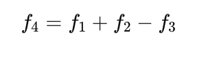
How Does the Refractive Index Play a Role?
The refractive index of the fiber is a measure of how much the light slows down as it passes through the fiber. Normally, this refractive index is constant. However, when the optical power is high, the refractive index becomes dependent on the intensity of the light.This relationship is given by:

Where:

The role of an Network Engineer is rapidly evolving with the increasing demand for automation to manage complex networks effectively. Whether you’re preparing for a job posting at Amazon Web Services (AWS) or Google or any other leading technology company, having a solid foundation in network engineering combined with proficiency in automation is essential. During my experience so far,I myself have appeared in multiple interviews and have interviewed multiple candidates where I have noticed that since most of the current networking companies have robust software infrastructure built already with software engineers ;network engineers either don’t have to write code or they don’t get chance to write script and codes. This makes them a bit hesitant answering automation related questions and some time even they say “I don’t know automation” which I feel not the right thing because I am sure they have either written a small macro in microsoft excel ,or a small script to perform some calculation, or a program to telnet device and do some operation.So be confident to realise your potential and ready to say “I have written few or small scripts that were needed to expedite my work but if it is needed to write some code with current profile ,I can ramp-up fast and can wrote as I am open to learn and explore more after all its just a language to communicate to machine to perform some task and its learnable”.
This article provides foundational information on Python programming, focusing on lists, dictionaries, tuples, mutability, loops, and more, to help you prepare for roles that require both network engineering knowledge and automation skills.
An Network Engineer typically handles the following responsibilities:
- Design and Implementation: Build and deploy networking devices like optical, switches ,routers etc, including DWDM,IP-MPLS,OSPF,BGP etc and other advanced technologies.
- Network Scaling: Enhance and scale network designs to meet increasing demands.
- Process Development: Create and refine processes for network operation and deployment.
- Cross-Department Collaboration: Work with other teams to design and implement network solutions.
- Standards Compliance: Ensure network adherence to industry and company standards.
- Change Management: Review and implement network changes to improve performance and reliability.
- Operational Excellence: Lead projects to enhance network quality and dependability.
- Problem-Solving and Innovation: Troubleshoot complex issues and develop innovative solutions for network challenges.
Preparing for the Interview
Understanding Core or Leadership Principles
Many companies, like AWS, Google emphasize specific leadership principles or core values. Reflect on your experiences and prepare to discuss how you have applied these principles in your work. Last year I wrote an article in reference to AWS which you can visit here
Some of the common Leadership Principles or core/mission values are
- https://www.amazon.jobs/content/en/our-workplace/leadership-principles
- https://about.google/philosophy/
Behavioural Interview Questions
Expect behavioural questions that assess your problem-solving skills and past experiences. Use the STAR method (Situation, Task, Action, Result) to structure your responses.Most of the fair hire companies will have page dedicated to their hiring process which I will strongly encourage everyone to visit their page like
- https://aws.amazon.com/careers/how-we-hire/
- https://www.google.com/about/careers/applications/interview-tips/
- https://www.metacareers.com/swe-prep-onsite/
Now lets dive into the important piece of this article because we are still a little far from the point where nobody needs to write code but AI will do all necessary code for users by basic autosuggestions statements.
Automation Warm-up session
Pretty much every service provider is using python at this point of time so lets get to know some of the things that will build readers foundation and remove the fear to appear for interviews that has automation as core skill. Just prepare these by heart and I can assure you will do good with the interviews
1. Variables and Data Types
Variables store information that can be used and manipulated in your code. Python supports various data types, including integers, floats, strings, and booleans.
# Variables and data types
device_name = "Router1"  # String
status = "Active"  # String
port_count = 24  # Integer
error_rate = 0.01  # Float
is_operational = True  # Boolean

print(f"Device: {device_name}, Status: {status}, Ports: {port_count}, Error Rate: {error_rate}, Operational: {is_operational}")
2. Lists
Lists are mutable sequences that can store a collection of items. Lists allow you to store and manipulate a collection of items.
# Creating and manipulating lists
devices = ["Router1", "Switch1", "Router2", "Switch2"]

# Accessing list elements
print(devices[0])  # Output: Router1

# Adding an element
devices.append("Router3")
print(devices)  # Output: ["Router1", "Switch1", "Router2", "Switch2", "Router3"]

# Removing an element
devices.remove("Switch1")
print(devices)  # Output: ["Router1", "Router2", "Switch2", "Router3"]

# Iterating through a list
for device in devices:
    print(device)
3. Dictionaries
# Creating and manipulating dictionaries
device_statuses = {
    "Router1": "Active",
    "Switch1": "Inactive",
    "Router2": "Active",
    "Switch2": "Active"
}

# Accessing dictionary values
print(device_statuses["Router1"])  # Output: Active

# Adding a key-value pair
device_statuses["Router3"] = "Active"
print(device_statuses)  # Output: {"Router1": "Active", "Switch1": "Inactive", "Router2": "Active", "Switch2": "Active", "Router3": "Active"}

# Removing a key-value pair
del device_statuses["Switch1"]
print(device_statuses)  # Output: {"Router1": "Active", "Router2": "Active", "Switch2": "Active", "Router3": "Active"}

# Iterating through a dictionary
for device, status in device_statuses.items():
    print(f"Device: {device}, Status: {status}")
Dictionaries are mutable collections that store items in key-value pairs. They are useful for storing related data.
4. Tuples
Tuples are immutable sequences, meaning their contents cannot be changed after creation. They are useful for storing fixed collections of items.
# Creating and using tuples
network_segment = ("192.168.1.0", "255.255.255.0")

# Accessing tuple elements
print(network_segment[0])  # Output: 192.168.1.0

# Tuples are immutable
# network_segment[0] = "192.168.2.0"  # This will raise an error
5. Mutability and Immutability
Understanding the concept of mutability and immutability is crucial for effective programming.
- Mutable objects: Can be changed after creation (e.g., lists, dictionaries).
- Immutable objects: Cannot be changed after creation (e.g., tuples, strings).
# Example of mutability
devices = ["Router1", "Switch1"]
devices.append("Router2")
print(devices)  # Output: ["Router1", "Switch1", "Router2"]

# Example of immutability
network_segment = ("192.168.1.0", "255.255.255.0")
# network_segment[0] = "192.168.2.0"  # This will raise an error
6. Conditional Statements and Loops
Control the flow of your program using conditional statements and loops.
# Conditional statements
device = "Router1"
status = "Active"

if status == "Active":
    print(f"{device} is operational.")
else:
    print(f"{device} is not operational.")

# Loops
# For loop
for device in devices:
    print(device)

# While loop
count = 0
while count < 3:
    print(count)
    count += 1
7. Functions
Functions are reusable blocks of code that perform a specific task.
# Defining and using functions
def check_device_status(device, status):
    if status == "Active":
        return f"{device} is operational."
    else:
        return f"{device} is not operational."

# Calling a function
result = check_device_status("Router1", "Active")
print(result)  # Output: Router1 is operational.
8. File Handling
Reading from and writing to files is essential for automating tasks that involve data storage.
# Writing to a file
with open("device_statuses.txt", "w") as file:
    for device, status in device_statuses.items():
        file.write(f"{device}: {status}\n")

# Reading from a file
with open("device_statuses.txt", "r") as file:
    content = file.read()
    print(content)
9. Using Libraries
Python libraries extend the functionality of your code. For network automation, libraries like paramiko and netmiko are invaluable.
# Using the json library to work with JSON data
import json

# Convert dictionary to JSON
device_statuses_json = json.dumps(device_statuses)
print(device_statuses_json)

# Parse JSON back to dictionary
parsed_device_statuses = json.loads(device_statuses_json)
print(parsed_device_statuses)
Advanced Python for Network Automation
1. Network Automation Libraries
Utilize libraries such as paramiko for SSH connections, netmiko for multi-vendor device connections, and pyntc for network management.
2. Automating SSH with Paramiko
import paramiko

def ssh_to_device(ip, username, password, command):
    ssh = paramiko.SSHClient()
    ssh.set_missing_host_key_policy(paramiko.AutoAddPolicy())
    ssh.connect(ip, username=username, password=password)
    stdin, stdout, stderr = ssh.exec_command(command)
    return stdout.read().decode()

# Example usage
output = ssh_to_device("192.168.1.1", "admin", "password", "show ip interface brief")
print(output)
3. Automating Network Configuration with Netmiko
from netmiko import ConnectHandler

device = {
    'device_type': 'cisco_ios',
    'host': '192.168.1.1',
    'username': 'admin',
    'password': 'password',
}

net_connect = ConnectHandler(**device)
output = net_connect.send_command("show ip interface brief")
print(output)
4. Using Telnet with telnetlib
import telnetlib

def telnet_to_device(host, port, username, password, command):
    try:
        # Connect to the device
        tn = telnetlib.Telnet(host, port)

        # Read until the login prompt
        tn.read_until(b"login: ")
        tn.write(username.encode('ascii') + b"\n")

        # Read until the password prompt
        tn.read_until(b"Password: ")
        tn.write(password.encode('ascii') + b"\n")

        # Execute the command
        tn.write(command.encode('ascii') + b"\n")

        # Wait for command execution and read the output
        output = tn.read_all().decode('ascii')

        # Close the connection
        tn.close()

        return output
    except Exception as e:
        return str(e)

# Example usage
host = "192.168.1.1"
port = 3083
username = "admin"
password = "password"
command = "rtrv-alm-all:::123;"

output = telnet_to_device(host, port, username, password, command)
print(output)
5. Using SSH with paramiko
import paramiko

def ssh_to_device(host, port, username, password, command):
    try:
        # Create an SSH client
        ssh = paramiko.SSHClient()

        # Automatically add the device's host key (not recommended for production)
        ssh.set_missing_host_key_policy(paramiko.AutoAddPolicy())

        # Connect to the device
        ssh.connect(host, port=port, username=username, password=password)

        # Execute the command
        stdin, stdout, stderr = ssh.exec_command(command)

        # Read the command output
        output = stdout.read().decode()

        # Close the connection
        ssh.close()

        return output
    except Exception as e:
        return str(e)

# Example usage
host = "192.168.1.1"
port = 3083
username = "admin"
password = "password"
command = "rtrv-alm-all:::123;"

output = ssh_to_device(host, port, username, password, command)
print(output)
6. Using Telnet with telnetlib with list of devices.
import telnetlib

def telnet_to_device(host, port, username, password, command):
    try:
        # Connect to the device
        tn = telnetlib.Telnet(host, port)

        # Read until the login prompt
        tn.read_until(b"login: ")
        tn.write(username.encode('ascii') + b"\n")

        # Read until the password prompt
        tn.read_until(b"Password: ")
        tn.write(password.encode('ascii') + b"\n")

        # Execute the command
        tn.write(command.encode('ascii') + b"\n")

        # Wait for command execution and read the output
        output = tn.read_all().decode('ascii')

        # Close the connection
        tn.close()

        return output
    except Exception as e:
        return str(e)

# List of devices
devices = [
    {"host": "192.168.1.1", "port": 3083, "username": "admin", "password": "password"},
    {"host": "192.168.1.2", "port": 3083, "username": "admin", "password": "password"},
    {"host": "192.168.1.3", "port": 3083, "username": "admin", "password": "password"}
]

command = "rtrv-alm-all:::123;"

# Execute command on each device
for device in devices:
    output = telnet_to_device(device["host"], device["port"], device["username"], device["password"], command)
    print(f"Output from {device['host']}:\n{output}\n")
or
import telnetlib

def telnet_to_device(host, port, username, password, command):
    try:
        # Connect to the device
        tn = telnetlib.Telnet(host, port)

        # Read until the login prompt
        tn.read_until(b"login: ")
        tn.write(username.encode('ascii') + b"\n")

        # Read until the password prompt
        tn.read_until(b"Password: ")
        tn.write(password.encode('ascii') + b"\n")

        # Execute the command
        tn.write(command.encode('ascii') + b"\n")

        # Wait for command execution and read the output
        output = tn.read_all().decode('ascii')

        # Close the connection
        tn.close()

        return output
    except Exception as e:
        return str(e)

# List of device IPs
device_ips = [
    "192.168.1.1",
    "192.168.1.2",
    "192.168.1.3"
]

# Common credentials and port
port = 3083
username = "admin"
password = "password"
command = "rtrv-alm-all:::123;"

# Execute command on each device
for ip in device_ips:
    output = telnet_to_device(ip, port, username, password, command)
    print(f"Output from {ip}:\n{output}\n")
7. Using SSH with paramiko with list of devices
import paramiko

def ssh_to_device(host, port, username, password, command):
    try:
        # Create an SSH client
        ssh = paramiko.SSHClient()

        # Automatically add the device's host key (not recommended for production)
        ssh.set_missing_host_key_policy(paramiko.AutoAddPolicy())

        # Connect to the device
        ssh.connect(host, port=port, username=username, password=password)

        # Execute the command
        stdin, stdout, stderr = ssh.exec_command(command)

        # Read the command output
        output = stdout.read().decode()

        # Close the connection
        ssh.close()

        return output
    except Exception as e:
        return str(e)

# List of devices
devices = [
    {"host": "192.168.1.1", "port": 3083, "username": "admin", "password": "password"},
    {"host": "192.168.1.2", "port": 3083, "username": "admin", "password": "password"},
    {"host": "192.168.1.3", "port": 3083, "username": "admin", "password": "password"}
]

command = "rtrv-alm-all:::123;"

# Execute command on each device
for device in devices:
    output = ssh_to_device(device["host"], device["port"], device["username"], device["password"], command)
    print(f"Output from {device['host']}:\n{output}\n")
or
import paramiko

def ssh_to_device(host, port, username, password, command):
    try:
        # Create an SSH client
        ssh = paramiko.SSHClient()

        # Automatically add the device's host key (not recommended for production)
        ssh.set_missing_host_key_policy(paramiko.AutoAddPolicy())

        # Connect to the device
        ssh.connect(host, port=port, username=username, password=password)

        # Execute the command
        stdin, stdout, stderr = ssh.exec_command(command)

        # Read the command output
        output = stdout.read().decode()

        # Close the connection
        ssh.close()

        return output
    except Exception as e:
        return str(e)

# List of device IPs
device_ips = [
    "192.168.1.1",
    "192.168.1.2",
    "192.168.1.3"
]

# Common credentials and port
port = 3083
username = "admin"
password = "password"
command = "rtrv-alm-all:::123;"

# Execute command on each device
for ip in device_ips:
    output = ssh_to_device(ip, port, username, password, command)
    print(f"Output from {ip}:\n{output}\n")
Proficiency in Python and understanding the foundational concepts of lists, dictionaries, tuples, mutability, loops, and functions are crucial for automating tasks in network engineering. By practising and mastering these skills, you can enhance your problem-solving capabilities, improve network efficiency, and contribute to innovative solutions within your organization.
This guide serves as a starting point for your preparation. Practice coding regularly, explore advanced topics, and stay updated with the latest advancements in network automation. With dedication and the right preparation, you’ll be well-equipped to excel in any network engineering role.
If you feel that any other information that can help you being reader and for others ,feel free to leave comment and I will try to incorporate those in future.
All the best!
References

Based on my experience ,I have seen that Optical Engineers need to estimate Optical Signal-to-Noise Ratio (OSNR) often specially when they are dealing with network planning and operations .Mostly engineers use spreadsheet to perform these calculation or use available planning tool .This handy tool provides a method for user to quickly estimate the OSNR for a link and ensures flexibility to simulate by modifying power levels,Tx OSNR, number of channels . In this blog post, I will walk you through the features and functionalities of the tool, helping you understand how to use it effectively for your projects.For simplicity ,we have not considered Non-Linear penalties which user is requested to add as needed .
What is OSNR?
Optical Signal-to-Noise Ratio (OSNR) is a critical parameter in optical communication systems. It measures the ratio of signal power to the noise power in an optical channel. Higher OSNR values indicate better signal quality and, consequently, better performance of the communication system.
Features of the OSNR Simulation Tool
This OSNR Calculation Tool is designed to simplify the process of calculating the OSNR across multiple channels and Intermediate Line Amplifiers (ILAs). Here’s what the tool offers:
-
Input Fields for Channels, Tx OSNR, and Number of ILAs:
-
-
-
-
-
- Channels: The number of optical channels in the network. Adjust to simulate different network setups.
- Tx OSNR: The initial OSNR value at the transmitter.
- Number of ILAs: The number of in-line amplifiers (ILAs) in the network. Adjust to add or remove amplifiers.
- Set Noise Figure (dB) for all ILAs: Set a common noise figure for all ILAs.
- Margin: The margin value used for determining if the final OSNR is acceptable.
- Set Pin_Composite (dBm) for all: Set a common Pin_Composite (dBm) value for all components.
- BitRate: Controlled via a slider. Adjust the slider to select the desired bit rate.
- BaudRate: Automatically updated based on the selected bit rate.
- ROSNR: Automatically updated based on the selected bit rate.
- RSNR: Automatically updated based on the selected bit rate.
- Baud Rate: Additional input for manual baud rate entry.
-
-
-
-
-
-
Dynamic ILA Table Generation:
-
-
-
-
-
- The tool generates a table based on the number of ILAs specified. This table includes fields for each component (TerminalA, ILAs, TerminalZ) with editable input fields for Pin_Composite (dBm) and Noise Figure (dB).
-
-
-
-
-
-
Calculations and Outputs:
-
-
-
-
-
- Composite Power: The composite power calculated based on the number of channels and per-channel power.
- Net Power Change: The net power change when channels are added or removed.
- Optical Parameter Conversions:
- Frequency to Wavelength and vice versa.
- Power in mW to dBm and vice versa.
- Coupling Ratio to Insertion Loss and vice versa.
- OSNR (dB): Displays the OSNR value for each component in the network.
- RSNR (dB): Displays the RSNR value for each component in the network.
-
-
-
-
-
-
Baud Rate and Required SNR Calculation:
-
-
-
-
-
- Input the Baud Rate to calculate the required Signal-to-Noise Ratio (SNR) for your system.SNR is related to Q-factor .
-
-
-
-
-
-
Reset to Default:
-
-
-
-
-
- A button to reset all fields to their default values for a fresh start.
-
-
-
-
-
Steps to Use the Tool
- Set the Initial Parameters:
-
-
-
-
- Enter the number of channels.
- Enter the Tx OSNR value.
- Enter the number of ILAs.
- Optionally, set a common Noise Figure for all ILAs.
- Enter the margin value.
- Optionally, set a common Pin_Composite (dBm) for all components.
-
-
-
-
- Adjust Bit Rate:
-
-
-
-
- Use the slider to select the desired bit rate. The BaudRate, ROSNR, and RSNR will update automatically.
-
-
-
-
- Calculate:
-
-
-
-
- The tool will automatically calculate and display the OSNR and RSNR values for each component.
-
-
-
-
- Review Outputs:
-
-
-
-
- Check the Composite Power, Net Power Change, and Optical Parameter Conversions.
- Review the OSNR and RSNR values.
- The final OSNR value will be highlighted in green if it meets the design criteria (OSNR >= ROSNR + Margin), otherwise, it will be highlighted in red.
-
-
-
-
- Visualize:
-
-
-
- The OSNR vs Components chart will provide a visual representation of the OSNR values across the network components.
-
-
-
- Reset to Default:
-
-
-
-
- Use the “Reset to Default” button to reset all values to their default settings.
-
-
-
-
Themes
You can change the visual theme of the tool using the theme selector dropdown. Available themes include:
-
-
-
-
- Default
- Theme 1
- Theme 2
- Theme 3
- Theme 4
-
-
-
Each theme will update the colors and styles of the tool to suit your preferences.
Notes:
- Editable fields are highlighted in light green. Adjust these values as needed.
- The final OSNR value’s background color will indicate if the design is acceptable:
- Green: OSNR meets or exceeds the required margin.
- Red: OSNR does not meet the required margin.
Formulas used:
Composite Power Calculation
Composite Power (dBm)=Per Channel Power (dBm)+10log10(Total number of channels − Insertion Loss of Filter (dB)
Net Power Change Calculation
Net Power Change (dBm)=10log10(Channels added/removed+Channels undisturbed)−10log10(Channels undisturbed)
Optical Parameter Conversions

OSNR Calculation

RSNR Calculation

Shannon Capacity Formula
To calculate the required SNR given bit rate and baud rate:
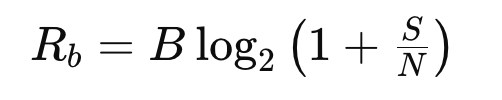
Rearranged to solve for SNR:
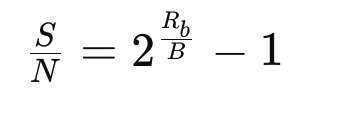
Example Calculation
Given Data:
- Bit Rate (Rb): 200 Gbps
- Baud Rate (Bd): 69.40 Gbaud
Example Tool Usage
Suppose you are working on a project with the following specifications:
-
-
-
-
-
- Channels: 4
- Tx OSNR: 35 dB
- Number of ILAs: 4
-
-
-
-
- Enter these values in the input fields. (whatever is green is editable)
- The tool will generate a table with columns for TerminalA, ILA1, ILA2, ILA3, ILA4, and TerminalZ.
- Adjust the Pin_Composite (dBm) and Noise Figure (dB) values if necessary.
- The tool calculates the Pin_PerChannel (dBm) and OSNR for each component, displaying the final OSNR at TerminalZ.
- Input the Baud Rate to calculate the required SNR
- User can see the OSNR variation at each component level(ILA here) to see the variation.

The integration of artificial intelligence (AI) into optical networking is set to dramatically transform offering numerous benefits for engineers at all levels of expertise. From automating routine tasks to enhancing network performance and reliability, AI promises to make the lives of optical networking engineers easier and more productive. Here’s a detailed look at how AI is transforming this industry.

Automation and Efficiency
One of the most significant ways AI is enhancing optical networking is through automation. Routine tasks such as network monitoring, fault detection, and performance optimization can be automated using AI algorithms. This allows engineers to focus on more complex and innovative aspects of network management. AI-driven automation tools can identify and predict network issues before they become critical, reducing downtime and maintenance costs.Companies like Cisco are implementing AIOps (Artificial Intelligence for IT Operations), which leverages machine learning to streamline IT operations. This involves using AI to analyse data from network devices, predict potential failures, and automate remediation processes. Such systems provide increased visibility into network operations, enabling quicker decision-making and problem resolution
Enhanced Network Performance
AI can significantly enhance network performance by optimising traffic flow and resource allocation. AI algorithms analyse vast amounts of data to understand network usage patterns and adjust resources dynamically. This leads to more efficient utilisation of bandwidth and improved overall network performance . Advanced AI models can predict traffic congestion and reroute data to prevent bottlenecks. For instance, in data centers where AI and machine learning workloads are prevalent, AI can manage data flow to ensure that high-priority tasks receive the necessary bandwidth, thereby improving processing efficiency and reducing latency
Predictive Maintenance
AI’s predictive capabilities are invaluable in maintaining optical networks. By analysing historical data and identifying patterns, AI can predict when and where equipment failures are likely to occur. This proactive approach allows for maintenance to be scheduled during non-peak times, minimising disruption to services Using AI, engineers can monitor the health of optical transceivers and other critical components in real-time. Predictive analytics can forecast potential failures, enabling preemptive replacement of components before they fail, thus ensuring continuous network availability .
Improved Security
AI enhances the security of optical networks by detecting and mitigating threats in real-time. Machine learning algorithms can identify unusual network behavior that may indicate a security breach, allowing for immediate response to potential threats.AI-driven security systems can analyse network traffic to identify patterns indicative of cyber-attacks. These systems can automatically implement countermeasures to protect the network, significantly reducing the risk of data breaches and other security incidents.
Bridging the Skills Gap
For aspiring optical engineers, AI can serve as a powerful educational tool. AI-powered simulation and training programs can provide hands-on experience with network design, deployment, and troubleshooting. This helps bridge the skills gap and prepares new engineers to handle complex optical networking tasks Educational institutions and training providers are leveraging AI to create immersive learning environments. These platforms can simulate real-world network scenarios, allowing students to practice and hone their skills in a controlled setting before applying them in the field .
Future Trends
Looking ahead, the role of AI in optical networking will continue to expand. Innovations such as 800G pluggables and 1.6T coherent optical engines are on the horizon, promising to push network capacity to new heights. As optical networking technology continues to advance, AI will play an increasingly central role. From managing ever-growing data flows to ensuring the highest levels of network security, AI tools offer unprecedented advantages. The integration of AI into optical networking promises not only to improve the quality of network services but also to redefine the role of the network engineer. With AI’s potential still unfolding, the future holds exciting prospects for innovation and efficiency in optical networking.
References:

Navigating a job interview successfully is crucial for any job seeker looking to make a positive impression. This often intimidating process can be transformed into an empowering opportunity to showcase your strengths and fit for the role. Here are refined strategies and insights to help you excel in your next job interview.
1. Focus on Positive Self-Representation
When asked to “tell me about yourself,” this is your chance to control the narrative. This question is a golden opportunity to succinctly present yourself by focusing on attributes that align closely with the job requirements and the company’s culture. Begin by identifying your key personality traits and how they enhance your professional capabilities. Consider what the company values and how your experiences and strengths play into these areas. Practicing your delivery can boost your confidence, enabling you to articulate a clear and focused response that demonstrates your suitability for the role. For example, explaining how your collaborative nature and creativity in problem-solving match the company’s emphasis on teamwork and innovation can set a strong tone for the interview.
2. Utilize the Power of Storytelling
Personal stories are not just engaging; they are a compelling way to illustrate your skills and character to the interviewer. Think about your past professional experiences and select stories that reflect the qualities the employer is seeking. These narratives should go beyond simply stating facts; they should convey your personal values, decision-making processes, and the impact of your actions. Reflect on challenges you’ve faced and how you’ve overcome them, focusing on the insights gained and the results driven. This method helps the interviewer see beyond your resume to the person behind the accomplishments.
3. Demonstrate Vulnerability and Growth
It’s important to be seen as approachable and self-aware, which means acknowledging not just successes but also vulnerabilities. Discussing a past failure or challenge and detailing what you learned from it can significantly enhance your credibility. This openness shows that you are capable of self-reflection and willing to grow from your experiences. Employers value candidates who are not only skilled but are also resilient and ready to adapt based on past lessons.
4. Showcase Your Authentic Self
Authenticity is key in interviews. It’s essential to present yourself truthfully in terms of your values, preferences, and style. This could relate to your cultural background, lifestyle choices, or personal philosophies. A company that respects and values diversity will appreciate this honesty and is more likely to be a good fit for you in the long term. Displaying your true self can also help you feel more at ease during the interview process, as it reduces the pressure to conform to an idealized image.
5. Engage with Thoughtful Questions
Asking insightful questions during an interview can set you apart from other candidates. It shows that you are thoughtful and have a genuine interest in the role and the company. Inquire about the team dynamics, the company’s approach to feedback and growth, and the challenges currently facing the department. These questions can reveal a lot about the internal workings of the company and help you determine if the environment aligns with your professional goals and values.
Conclusion
Preparing for a job interview involves more than rehearsing standard questions; it requires a strategic approach to how you present your professional narrative. By emphasising a positive self-presentation, employing storytelling, showing vulnerability, maintaining authenticity, and asking engaging questions, you can make a strong impression. Each interview is an opportunity not only to showcase your qualifications but also to find a role and an organisation where you can thrive and grow.
References
- Self experience
- Internet
- hbr