
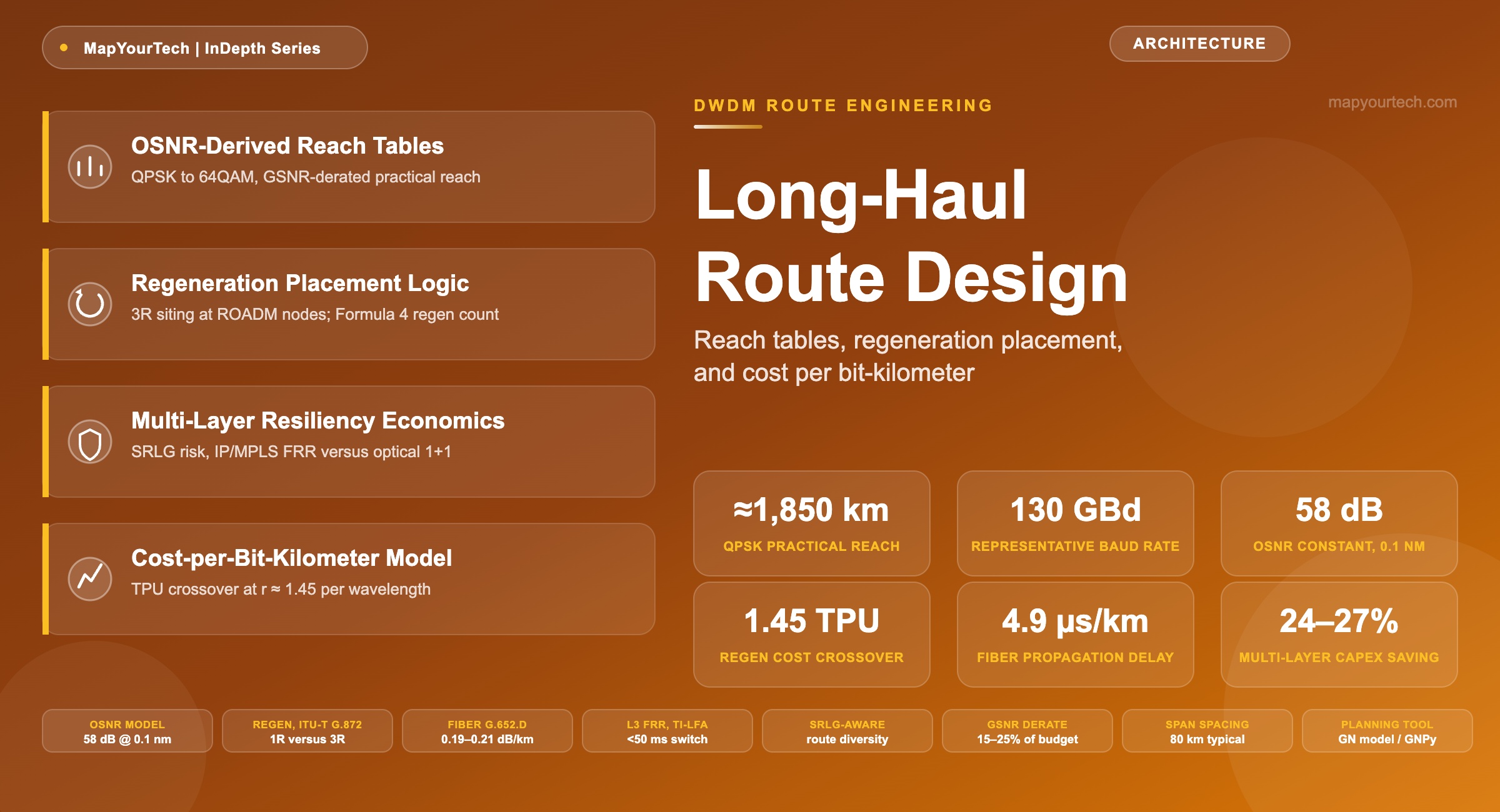
Long-Haul Route Design: Reach Tables, Regen Placement, and Cost per Bit-Kilometer
A route-engineering method that turns fiber characterization, OSNR budgets, and protection choices into a defensible reach table, a regeneration plan, and a cost-per-bit-kilometer number an operator can act on.
1. Introduction
A long-haul route design starts with three numbers an operator already has — the fiber path length, the ring or mesh topology it must join, and the capacity a sales team has promised a customer — and ends with a bill of materials: how many amplifier huts, how many regeneration sites, what modulation format runs on each segment, and what it all costs per bit carried per kilometer. Everything between those two points is physics and arithmetic, and the goal of this article is to make that arithmetic explicit enough to repeat on a different route without guessing.
The method has four moving parts that depend on each other in a fixed order. The fiber plant and the amplifier chain set an optical signal-to-noise ratio (OSNR) budget. That budget, applied against the OSNR requirement of each modulation format, produces a reach table — the maximum unregenerated distance for each capacity point. Comparing the reach table against the actual route length tells an engineer where regeneration sites are unavoidable and how many. Protection strategy then multiplies the working capacity by an overhead factor that depends on the resiliency tier the service requires. The sum of all of it, divided by capacity and by distance, is the cost-per-bit-kilometer figure that decides whether a route is worth building at all.
This piece works through each stage with the formulas shown, states every assumption in the worked examples, and closes with a full numeric case study on a 2,400 km route so the method can be checked end to end rather than taken on faith. It assumes familiarity with coherent DWDM fundamentals — modulation formats, EDFA and Raman amplification, and basic link-budget arithmetic — and builds directly on top of them.
Scope. This article covers terrestrial long-haul route design — roughly 500 to 3,000 km point-to-point or mesh segments carried on standard single-mode fiber with EDFA and hybrid Raman amplification. Submarine cable systems share the same OSNR and GSNR mathematics but differ enough in repeater design, powering, and 25-year lifetime margining that they are treated separately in the submarine repeater and unrepeatered systems literature referenced along the way.
The stakes of getting this sequence right are not abstract. A route provisioned with the wrong modulation format discovers the mistake only when a wavelength that tested clean in the lab fails to close its OSNR budget once real fiber aging and a handful of unplanned repair splices are added — usually months after commissioning, when the fix is a costly field visit rather than a spreadsheet correction. A route that under-counts regeneration sites at the design stage either ships with a capacity shortfall relative to what was sold, or absorbs an unplanned regen build mid-deployment at a cost and schedule impact the original business case never priced in. Working through the method once, with every assumption stated, is materially cheaper than discovering the same physics in the field.
2. Fiber Plant and Route Characterization
Route design begins with what is already in the ground, not with what an engineer would prefer to have. A route characterization survey records span-by-span fiber length, splice and connector loss, fiber type, and the location of every existing amplifier hut or duct-access point, because those locations constrain where new equipment can practically go. Inline amplifier huts along established long-haul corridors were frequently built decades ago along roadsides and railroad rights-of-way, and a new design that ignores them in favor of a mathematically ideal 80 km spacing usually costs more than one that reuses them.
Fiber type and its effect on reach
The fiber type sets two numbers that the rest of the design chain depends on: attenuation (dB/km) and effective area (µm²). ITU-T G.652.D remains the most widely deployed long-haul fiber and the default assumption unless a route survey states otherwise. ITU-T G.654.E — large effective area, low-loss fiber originally developed for submarine use — has moved into terrestrial long-haul builds where its larger effective area suppresses nonlinear interference and its lower attenuation coefficient extends unregenerated reach at the cost of higher deployment expense and reduced bend tolerance.
| Fiber type | Standard | Attenuation (dB/km, C-band) | Effective area (µm²) | Typical role |
|---|---|---|---|---|
| Standard single-mode | ITU-T G.652.D | 0.19–0.21 | ~80 | Default long-haul and metro fiber; largest installed base |
| Non-zero dispersion-shifted | ITU-T G.655 | 0.20–0.22 | ~55–70 | Legacy long-haul builds; largely superseded by G.652.D for new coherent deployments |
| Large effective area, low-loss | ITU-T G.654.E | 0.16–0.18 | ~110–130 | New-build long-haul and submarine-derived terrestrial routes; extends reach and raises nonlinear threshold |
| Cutoff-shifted | ITU-T G.654.B | 0.18–0.20 | ~110–115 | Repeatered submarine and some ultra-long terrestrial spans |
Standard-specified: fiber classes and cutoff wavelengths per ITU-T G.652 and G.654. Attenuation and effective area figures are representative measured ranges for commercially deployed fiber of each class; a specific manufacturer's data sheet should be used for final design.
Span loss and the route survey
Span loss is not simply attenuation coefficient times span length. A real span carries splice loss roughly every 2 to 4 km of cable reel length (0.05–0.1 dB per splice), connector loss at every patch point (0.2–0.5 dB per mated pair), and a design margin for cable aging and repair splices over the system's operating life. A route survey that reports only "fiber attenuation × distance" without these additions routinely understates span loss by 2 to 4 dB across an 80 km span — enough to shift a modulation-format decision in the reach table two sections down.
L_span = α × L_km + N_splice × L_splice + N_conn × L_conn + M_cable
Practical Example An 80 km span of G.652.D fiber (α = 0.20 dB/km) with 22 factory splices at 0.08 dB each, two connector pairs at 0.3 dB each, and a 1.5 dB cable-aging margin: L_span = (0.20 × 80) + (22 × 0.08) + (2 × 0.3) + 1.5 = 16.0 + 1.76 + 0.6 + 1.5 = 19.86 dB, commonly rounded to 20 dB for planning. That 4 dB of non-attenuation loss is what a naive "α × distance" estimate misses.
Read the Full Analysis with Premium
The remaining 89% of this article — the design numbers, trade-offs and field guidance — is part of MapYourTech Premium, along with the full premium library, courses and professional tools.
You May Also Like

-
Free
-
September 4, 2026

-
Premium
-
September 4, 2026

-
Premium
-
September 4, 2026