
Generic selectors
Exact matches only
Search in title
Search in content
Post Type Selectors
Articles
lp_course
lp_lesson
Back
HomeFundamentalsRaman Engineering Deep Dive: Pump Plans, Gain Profiles, and Field Safety
Raman-Engineering-Deep-Dive-featured-image_09_07_2026_20_02_36

Raman Engineering Deep Dive: Pump Plans, Gain Profiles, and Field Safety

29 min read
4
Raman Engineering Deep Dive: Pump Plans and Field Safety
Skip to main content
MapYourTech | InDepth Series

Raman Engineering Deep Dive: Pump Plans, Gain Profiles, and Field Safety

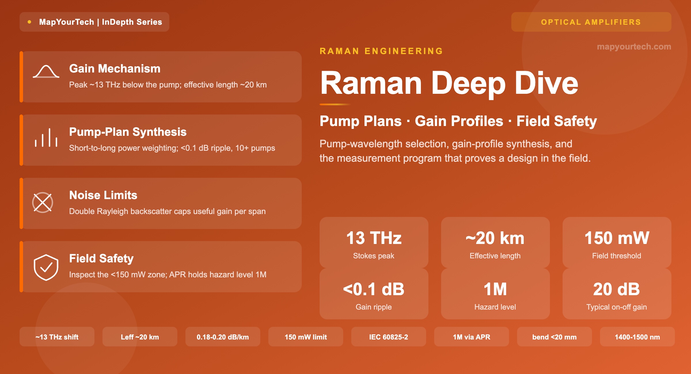
Pump-wavelength selection, gain-profile synthesis, and safety engineering — with worked pump plans for representative span classes and the measurement program that proves a design in the field.

FocusDistributed Raman
LevelAdvanced
BandsC + L, multi-band
StandardsITU-T, IEC 60825-2

1. Introduction

A distributed Raman amplifier turns the span fiber itself into gain medium. You launch one or more high-power pumps in the 1,400–1,500 nm region, and stimulated Raman scattering transfers pump photons to signal photons roughly 13 THz lower in frequency, along tens of kilometers of the deployed fiber. Nothing is doped, nothing is added at mid-span — the gain lives in the glass that was already in the ground. That single fact is what makes Raman worth the engineering effort: the signal is amplified before it has fully decayed, so the optical signal-to-noise ratio (OSNR) at the receiver is higher than any lumped amplifier at the end of the same span could deliver.

The cost of that benefit is a set of engineering problems an erbium-doped fiber amplifier (EDFA) never presents. You are putting hundreds of milliwatts — sometimes more than a watt — into an installed fiber whose splice enclosures, connectors, and tight bends you cannot see. The gain shape depends on pump-to-pump power transfer that only a numerical solver predicts. Double Rayleigh backscatter, negligible in a doped amplifier, becomes the ceiling on how much gain you can safely take. And the pump light does not stop being dangerous at the equipment bulkhead — it travels down the span, so the hazard is a property of the outside plant, not the card.

This article treats Raman as a design discipline rather than a phenomenon. It moves from the gain mechanism and pump-plan synthesis, through the noise limits that bound useful gain, to the field-safety procedures that govern turn-up, and closes with the measurement program that proves a design once the fiber is in the ground. The worked pump plans are engineering examples grounded in the published physics, not vendor data sheets; where a specific product figure appears, it is labeled as a vendor claim and sourced. The physics is durable; the deployment context — C+L expansion, multi-band research, and AI-era data center interconnect — is current.

Who this is for

An engineer sizing a Raman stage for a long span, auditing a turn-up procedure, or trying to understand why a gain profile refuses to flatten. Foundations are explained as they arrive, so an early-career engineer can follow the mechanism while a system architect finds the trade-off boundaries stated explicitly.

2. The Gain Mechanism You Are Buying

Stimulated Raman scattering (SRS) is inelastic: a pump photon scatters off a molecular vibration (an optical phonon) in the silica and re-emits at lower energy, adding a photon to the signal field if a signal is present at that lower frequency. In germano-silicate transmission fiber the phonon spectrum is broad — it extends from zero to more than 26 THz — so gain is available at almost any signal wavelength provided you place a pump about one Stokes shift above it (measured on four fiber types, Headley and Agrawal). The consequence is the property that defines Raman as a technology: gain at any wavelength you choose, set by where you put the pump, not by a fixed material emission line.

The peak of that gain sits where the pump-to-signal frequency separation equals about 13 THz (measured; the gain spectrum recorded with a 1,425 nm pump on standard fiber types peaks near this offset). At 1,550 nm, 13 THz corresponds to a wavelength separation of roughly 100 nm, which is why C-band signals near 1,550 nm are pumped near 1,450 nm. Move the pump and the whole gain curve moves with it — the shape is a fiber property, the position is your choice.

Raman gain spectrum and Stokes shift A pump at about 1450 nm produces a broad Raman gain curve peaking about 13 THz lower in frequency, near 1550 nm, with usable gain spanning tens of nanometres. Signal frequency shift below pump (THz) Raman gain coefficient Peak ~13 THz 0 13 20 26 Pump ~1450 nm position is your choice C-band ~1550 nm signal receives gain here
Figure 1: The Raman gain curve is a fiber property; a pump near 1,450 nm places its ~13 THz peak on the C-band. A second bump near 26 THz carries little usable gain. Curve shape after measured spectra reported in the Raman amplification literature.

2.1 The gain coefficient and why effective area rules it

The single-pump signal evolution is a pair of coupled equations for signal and pump power. In the undepleted-pump regime — signal weak enough that it does not measurably drain the pump — the signal power at distance z has a closed form that every Raman calculation starts from.

On–off Raman gain, undepleted pump
Ps(z) = Ps(0) · exp( gR P0 Leff − αs z )
GA = Ps(L)pump on / Ps(L)pump off = exp( gR P0 Leff )
Leff = ( 1 − exp(−αp L) ) / αp

gR = Raman gain efficiency (W−1km−1); P0 = launched pump power (W); Leff = effective interaction length (km); αp, αs = fiber loss at pump and signal (km−1); L = span length (km). The on–off gain GA is what you measure by toggling the pump. Standard coupled-equation result (Headley and Agrawal).

Two design levers hide in that expression. The first is effective length: because the pump decays as it propagates, only the first 1/αp kilometers — roughly 20–22 km at typical 1,450 nm pump loss — contribute most of the interaction. Adding more span beyond that does not add proportional gain; it adds loss the pump has already stopped fighting. The second is the Raman gain efficiency gR, which scales inversely with the fiber's effective area. A dispersion-compensating fiber with a small core and high germanium content shows a gain coefficient several times that of large-area transmission fiber (measured across DCF, TrueWave RS, and pure-silica in the literature). That is why discrete Raman stages are often built on DCF: the same pump power buys far more gain in a small-area fiber. The boundary where this help stops is single-mode cutoff — shrink the core too far and the pump goes multimode, the overlap integral becomes ambiguous, and mode-dependent gain turns into a noise term.

Design boundary

Effective length caps the return on gain per span. Past roughly 20–22 km for a counter-pump, extra fiber contributes loss, not gain. This is why very long spans need either bidirectional pumping (attack the loss from both ends) or higher-order pumping (push gain deeper into the span), not simply more counter-pump power.

2.2 Polarization and the reason pumps are depolarized

Raman gain is polarization-dependent: a signal co-polarized with the pump sees markedly more gain than an orthogonal one. Left uncorrected, that produces polarization-dependent gain (PDG) that varies as the signal's state of polarization wanders, which appears as time-varying penalty at the receiver. The field fix is to depolarize the pump — either with an intrinsically unpolarized high-power source or by polarization-multiplexing two uncorrelated laser diodes — so the gain becomes the average of the co- and cross-polarized curves and the PDG collapses. Every practical distributed Raman pump is depolarized for this reason.

Takeaway: Raman gives gain at a wavelength you select rather than one a dopant fixes, with the peak about 13 THz below the pump and the efficiency set by effective area. Effective length — roughly the first 20 km — is where the pump does its work, and that geometric fact drives every architecture choice that follows.

3. Pump Wavelength Selection and Gain-Profile Synthesis

A single pump gives a gain peak about 20 nm wide — enough for a narrow band, not enough for the C-band and nowhere near C+L. Broadband Raman gain is built by wavelength-division-multiplexing several pumps at different wavelengths, each contributing its own overlapping gain hump, so the composite spectrum can be shaped almost arbitrarily (the technique reported by Namiki and Emori). The design question is which wavelengths, at which powers, produce the target gain shape.

Two effects make this harder than stacking curves. First, the pumps interact: energy transfers from shorter-wavelength pumps to longer ones through the same Raman process that amplifies the signal, so the longest-wavelength pump arrives partly fed by the others while the shortest is depleted. In a simulated five-pump plan, the shortest pump wavelength suffers the largest attenuation along the span while the longest experiences net gain (measured/simulated on dispersion-shifted fiber). Second, the signal band itself carries SRS tilt — shorter-wavelength channels pump longer ones. A gain profile that looks flat on paper tilts once real channel loading is applied, which is why C+L design cannot be done band-by-band in isolation.

Composite Raman gain from multiple pump wavelengths Four pump wavelengths each contribute an overlapping gain hump; their sum forms a flat composite gain across the signal band. Power is weighted toward the shorter pumps because energy transfers to the longer pumps. Signal wavelength (nm) Gain (dB) Composite gain (flat target) P1 P2 P3 P4 highest power lowest power Power weighting is counter-intuitive Longest pump gives most gain but needs modest power — it is fed by the shorter pumps.
Figure 2: A flat broadband profile is the sum of overlapping single-pump humps. Because energy flows from short to long pump wavelengths, the launched-power distribution is weighted toward the shorter pumps even though the longest pump supplies most of the useful gain — a pattern reported for measured C+L pump plans.
Premium Article — Free 21% Preview

Read the Full Analysis with Premium

The remaining 79% of this article — the design numbers, trade-offs and field guidance — is part of MapYourTech Premium, along with the full premium library, courses and professional tools.

Instant access · Cancel anytime · 48-hour trial available
Sanjay Yadav

Optical Communications & Network Automation Expert | Author of 3 Books for Optical Engineers | Founder, MapYourTech

Optical networking engineer with nearly two decades of experience across DWDM, OTN, coherent optics, submarine systems, and cloud infrastructure. Founder of MapYourTech.

Follow on LinkedIn

You May Also Like

52 min read 12 0 Like The Submarine Cable Stack: Open Cables, GSNR, SDM and Power Skip to main content...
  • Free
  • July 10, 2026
32 min read 10 0 Like Coherent DSP Architecture: From ADC Samples to Client Bits MAPYOURTECH | COHERENT OPTICS DEEP...
  • Free
  • July 10, 2026
42 min read 13 0 Like Building an Optical NOC Dashboard with OpenConfig Telemetry Skip to main content MapYourTech |...
  • Free
  • July 10, 2026

Course Title

Course description and key highlights

Course Content

Course Details


