
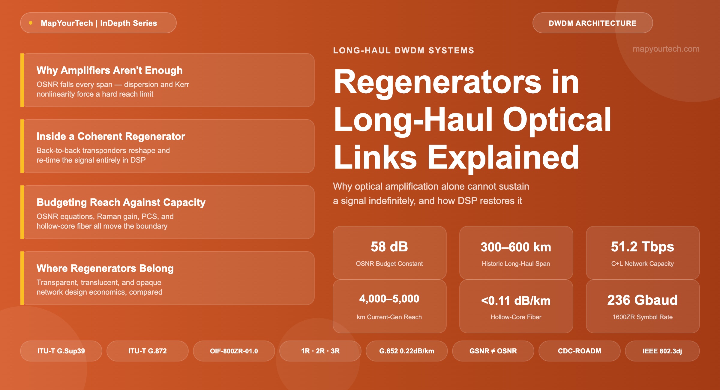
Regenerators in Long-Haul Optical Links Explained
Why an optical amplifier can never fully substitute for regeneration, how a modern coherent regenerator restores a signal at the bit level, and how network designers decide exactly where to spend the money.
1. Introduction
A 400 Gb/s wavelength riding a chain of erbium-doped fiber amplifiers (EDFAs) can travel a genuinely long way before it runs into trouble — but the trouble is not optional, and it does not announce itself gradually. Every amplifier in the chain restores the signal's power while adding amplified spontaneous emission (ASE) noise of its own, so the optical signal-to-noise ratio (OSNR) at the receiver keeps falling, span after span, with no natural floor. At some point on every long-haul route, that decline reaches the level where the forward error correction (FEC) in the receiving transponder can no longer close the link. The network then has exactly one option that is not an outage: stop the optical signal, convert it to electrical bits, clean it up completely, and re-launch it as a freshly generated optical signal on the next leg. That stop-clean-relaunch function is a regenerator, and deciding where a route needs one is one of the largest cost levers in long-haul network design.
This article works through that decision end to end. It starts with the physics that make regeneration unavoidable — ASE accumulation, chromatic and polarization-mode dispersion, and Kerr nonlinearity — and the ITU-T's formal distinction between 1R, 2R, and 3R regeneration. It then opens up what a modern regenerator actually contains: not a dedicated repeater box, but a back-to-back pair of coherent transponders with digital signal processing (DSP) doing the reshaping and retiming that used to require dedicated electronics. From there it moves into the design math — the OSNR budget equation that tells an engineer how many spans a given modulation format can survive — and into the mitigations that push the regenerator further down the route: Raman amplification, probabilistic constellation shaping, and simply choosing a lower-order modulation format. The article closes by comparing transparent, translucent, and opaque network philosophies, and by looking at where the OIF's 1600ZR/ZR+ and IEEE 802.3dj work is taking regenerator economics next.
The audience is anyone who has to answer a concrete version of this question for a real route: will this wavelength close without a mid-route conversion, and if not, where does the conversion belong? That question comes up identically whether you are sizing a single point-to-point link or building the routing and wavelength assignment (RWA) logic for a national mesh, and the physics underneath it does not change between the two.
2. Fundamentals of Optical Regeneration
What Regeneration Actually Restores
OSNR is the single number that determines whether a coherent receiver can lock onto a signal at all, and it only ever moves in one direction across a chain of optical amplifiers: down. ITU-T Supplement G.Sup39 (Optical system design and engineering considerations, edition 03/2025) formalizes this as noise concatenation: in a cascaded amplifier chain, ASE noise power adds from every stage, so OSNR degrades measurably after each amplifier regardless of how well that amplifier is designed. An EDFA or Raman amplifier restores optical power — it does nothing to remove noise that is already riding on the signal, and it introduces new noise of its own on every pass. That is the ceiling on what pure optical amplification can do, and it is the reason long-haul routes eventually need something categorically different from another amplifier.
The ITU-T draws the formal line in Annex A of ITU-T G.872, which G.Sup39 restates directly: 1R regeneration is power regeneration only — optical amplification plus, where present, dispersion compensation — and it is entirely analog, with no bit-level processing involved. 2R regeneration adds digital reshaping: the signal is detected, its amplitude decision is re-made, and a clean new waveform is generated. 3R regeneration goes one step further and adds re-timing — a recovered clock re-synchronizes the outgoing bit stream, removing accumulated timing jitter along with power loss and waveform distortion. The "R" in 1R/2R/3R stands for exactly that progression: regeneration of power, of power-and-shape, and of power-shape-and-timing. Only 2R and 3R require converting the signal out of the optical domain, which is why the industry shorthand for a regenerator is simply "O-E-O" — optical-to-electrical-to-optical.
| Class | What It Restores | Domain | Typical Realization |
|---|---|---|---|
| 1R | Signal power only (may include passive or amplifier-integrated dispersion compensation) | Optical / analog — no bit-level processing | In-line EDFA or Raman amplifier |
| 2R | Power and waveform shape (amplitude decision re-made) | Electrical / digital, via O-E-O — timing not re-synchronized | Legacy regenerator without clock recovery, largely historical in coherent-era networks |
| 3R | Power, shape, and timing — a newly generated signal, indistinguishable in quality from the original transmitter output | Electrical / digital, full O-E-O with recovered clock | Back-to-back coherent transponder pair with DSP and FEC |
Why the Line Moves: Dispersion and Nonlinearity
ASE accumulation is not the only impairment that eats into reach, though it is the one that never stops accumulating regardless of how carefully the system is engineered. Chromatic dispersion spreads pulses in time as different wavelength components travel at slightly different group velocities; in a coherent system this is compensated entirely in the digital domain, so it no longer forces a hard reach limit the way it did in direct-detection systems, but the DSP filter length — and therefore cost and power — scales with accumulated dispersion. Polarization-mode dispersion (PMD) adds a randomly time-varying penalty from birefringence in the fiber. Kerr nonlinearity — self-phase modulation, cross-phase modulation, and four-wave mixing — is different in kind: it grows with launch power, which means it cannot be fixed by simply turning the power up to compensate for span loss. Above a certain per-channel power, added power buys back OSNR at the cost of more nonlinear penalty, and the two effects trade off against each other around an optimum launch power. This optimum-power behavior is exactly what underlies the nonlinear Shannon limit for a fiber channel: achievable information rate rises with launch power in the ASE-limited regime, peaks, and then falls as nonlinearity dominates — a ceiling that no amount of receiver DSP can lift, because the penalty is added in the fiber itself before the signal ever reaches the receiver.
Read the Full Analysis with Premium
The remaining 87% of this article — the design numbers, trade-offs and field guidance — is part of MapYourTech Premium, along with the full premium library, courses and professional tools.
You May Also Like

-
Free
-
September 4, 2026

-
Premium
-
September 4, 2026

-
Premium
-
September 4, 2026