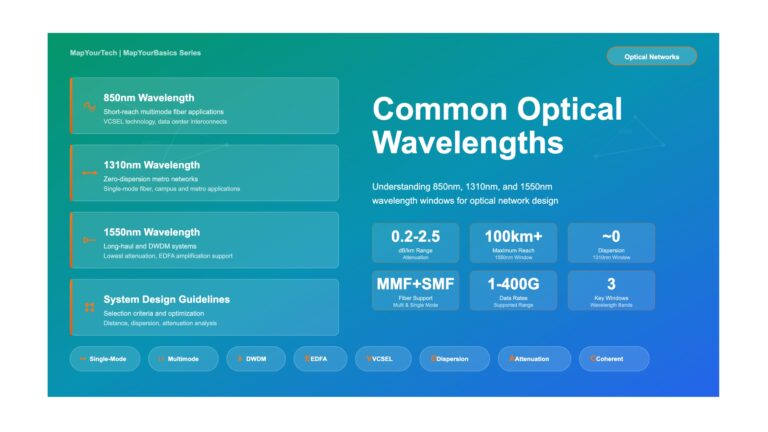
Common Optical Wavelengths: 850nm, 1310nm, 1550nm Use Cases and Technical Analysis Common Optical Wavelengths: 850nm, 1310nm, 1550nm Understanding wavelength windows,...
Digital Diagnostics Monitoring (DDM): Real-Time Transceiver Health Monitoring Digital Diagnostics Monitoring (DDM): Real-Time Transceiver Health Monitoring Comprehensive Guide to DDM/DOM...
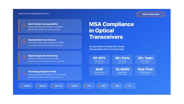
MSA Compliance in Optical Transceivers: Why Standards Are Essential MSA Compliance in Optical Transceivers: Why Standards Are Essential A Comprehensive...
PAM4 Modulation Explained: From NRZ to Multi-Level Signaling PAM4 Modulation Explained: From NRZ to Multi-Level Signaling A comprehensive technical exploration...
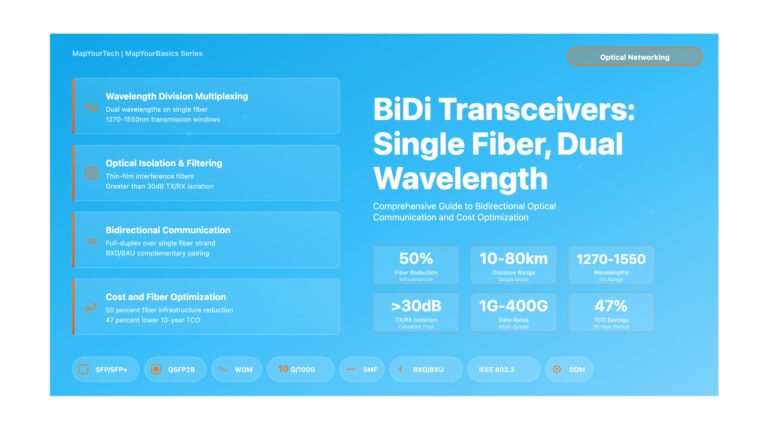
BiDi Transceivers: Single Fiber, Dual Wavelength Communication BiDi Transceivers: Single Fiber, Dual Wavelength Communication Comprehensive Guide to Bidirectional Optical Transmission...
Spatial Division Multiplexing (SDM) for Submarine Networks: Advanced Deep Dive Spatial Division Multiplexing (SDM) for Submarine Networks An Advanced Engineering...