
MapYourTech | InDepth Series
Optical Link Design Correlations: Interactive Engineering Reference
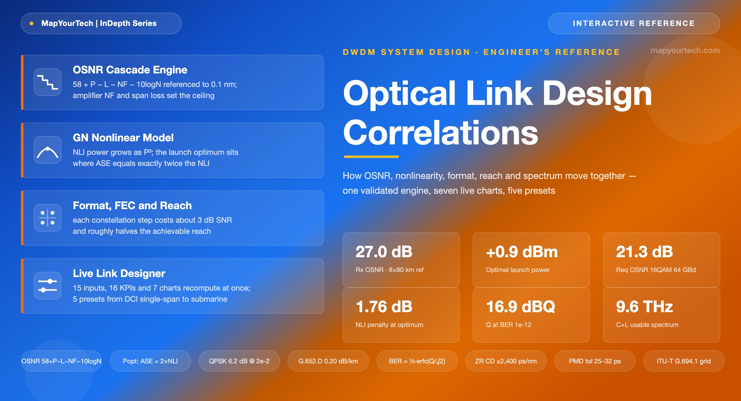
Every optical design decision moves at least three other numbers. This page wires the whole dependency chain into one live engine: launch power, span loss, noise figure, baud rate, modulation, FEC, fiber type and channel plan feed a cascade OSNR calculation and a GN-model nonlinear engine. Change any input below and watch margin, reach, capacity, dispersion budget and spectrum plan recompute across seven linked charts.
1. Introduction
An amplified coherent link is a closed system of trade-offs. Raise per-channel launch power by 1 dB and ASE-limited OSNR improves by 1 dB, but nonlinear interference rises by roughly 3 dB, so the effective SNR curve rolls over at an optimum that sits near −1 to +1 dBm per channel for 80 km spans of standard G.652.D fiber carrying 64 GBd signals. Double the span count and OSNR drops 3 dB, which costs one modulation step or half the capacity if the margin was already thin. Move from 64 GBd to 131 GBd at the same OSNR and the DSP sees about 3 dB less SNR, because the noise reference bandwidth of 0.1 nm stays fixed while the signal bandwidth doubles. None of these relationships is exotic, but they interact, and a designer who tracks them one at a time will miss the coupling that decides whether a wavelength closes. The foundational treatment of the noise side of this chain is in OSNR fundamentals for amplified links, and the tooling side of multivendor planning is covered in in-house optical link planning and simulation for operators.
This reference exists to make the coupling visible. Section 2 maps the dependency graph. Section 3 is the core: a full link designer whose inputs drive an OSNR cascade using the +58 planning formula and a Gaussian Noise (GN) model for nonlinear interference, with pass/warn/fail margin banding, an estimated pre-FEC BER, chromatic dispersion and PMD totals, one-way latency and per-fiber capacity. Sections 4 through 7 hold the supporting correlations an architect keeps reaching for: required OSNR versus baud rate per modulation format, reach versus format, CD accumulation against DSP tolerance windows, the Q-factor-to-BER curve with FEC thresholds, and channel-count-versus-spacing capacity across C, extended C and C+L bands. Section 8 collects the margin allocations and component ranges used in field planning.
Two conventions apply throughout. OSNR is always referenced to 0.1 nm (12.5 GHz at 1550 nm), and the OSNR-to-SNR conversion follows SNR = OSNR − 10·log10(Rs/12.5) with Rs in GBd, so a 131 GBd signal needs about 10.2 dB more OSNR than SNR for the same quality. Required-SNR values are computed from Gray-coded AWGN theory at the selected FEC threshold; the implementation-penalty input (default 1.5 dB) is where real DSPs, finite-length FEC and filtering live, and published transceiver datasheets typically sit 1 to 3 dB above the theory line. Where a figure is a spec-class or representative value rather than a physical constant, the page says so.
Read the Full Analysis with Premium
The remaining 88% of this article — the design numbers, trade-offs and field guidance — is part of MapYourTech Premium, along with the full premium library, courses and professional tools.
You May Also Like

-
Free
-
September 4, 2026

-
Premium
-
September 4, 2026

-
Premium
-
September 4, 2026