MapYourTech · MapYourBasics Series
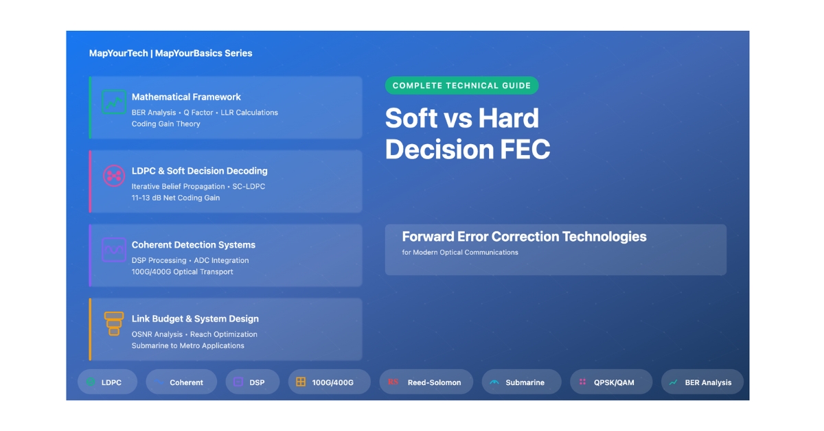
Soft vs Hard Decision FEC
The decoding choice that decides reach: whether the FEC sees a clean 1 or 0, or the receiver's soft reliability information — with the coding-gain math, the code families, the OSNR impact, and four calculators.
Introduction
Forward error correction adds redundancy so the receiver can fix errors without retransmission. The hard-versus-soft distinction is what the decoder is handed: a hard decoder gets only the sliced bit — a 1 or a 0, with the analog confidence thrown away — while a soft decoder keeps the quantized sample and its reliability and feeds that into iterative decoding. That extra information is worth roughly 2–3 dB of coding gain over a strong hard code at the same overhead, which is exactly the margin that turned 100G coherent and transoceanic reach into engineering rather than research. This guide builds the LLR and coding-gain math, surveys the code families from Reed-Solomon to spatially-coupled LDPC, quantifies the OSNR and reach impact, and provides four calculators.
The partial-credit analogy: a hard decision is a multiple-choice answer — the grader sees only A, B, C, or D. A soft decision shows the working, so a value that landed just past the threshold is marked "weakly a 1" rather than a confident 1, and the iterative decoder uses that across the codeword to recover bits a hard decoder would miss.
1. Fundamentals and Core Concepts
The hard decoder applies a threshold at the front end and decides each bit before FEC, discarding how far the sample sat from the threshold. The soft decoder skips that slice: it carries quantized samples with their statistics into the decoder and forms improved estimates. The physical reason soft FEC fits modern systems is that coherent detection already digitizes amplitude, phase, and both polarizations — the soft information is sitting in the ADC output for free.
The distinction matters most where every fraction of a dB counts: long-haul and submarine routes maximizing reach, 100G and above where OSNR targets are tight, coherent links where the soft data is already present, and higher-order modulation where the symbols sit closer together and noise sensitivity climbs. The payoff is concrete: lower amplifier count for a given reach, higher spectral efficiency, and the reach headroom that carried the industry from 10G direct-detect to 400G and 800G coherent.
2. Mathematical Framework
Hard-decision starting point: Q and BER
Q = (I₁ − I₀)/(σ₁ + σ₀) · BER = ½·erfc(Q/√2)
For Q > 7 the raw BER drops below 10⁻¹². Below that, the channel needs FEC to reach the 10⁻¹⁵ post-FEC target.
Practical Example — a pre-FEC operating point.
I₁ = 100 µA, I₀ = 20 µA, σ₁ = 10 µA, σ₀ = 5 µA: Q = 80/15 = 5.33; BER ≈ exp(−14.2)/(5.33·√2π) ≈ 5×10⁻⁸. That sits four orders of magnitude above the 10⁻¹² target — it is a normal raw channel that FEC must clean up, not an error-free link. A soft code with an ~11 dB net gain pulls a raw BER this size down past 10⁻¹⁵.
Soft-decision metric: log-likelihood ratio
L(z) = ln[ p(z | x=0) / p(z | x=1) ]; for AWGN BPSK, L = Lc·z, Lc = 2/σn²
The LLR encodes both the decision and its confidence in one signed number — large magnitude is a confident bit, near zero is a coin-flip. Iterative message passing exchanges these between variable and check nodes until the codeword converges.
Coding gain and overhead
NCG = coding gain − 10·log₁₀(1 + overhead) · effective rate = line rate / (1 + overhead)
The overhead is not free spectrum — it raises the symbol rate, so the net coding gain subtracts that penalty from the raw gain. A 20% overhead costs about 0.8 dB, which a soft code's raw gain absorbs easily.
Reach impact, done correctly
How extra coding gain converts to reach depends on the regime. On a loss-limited unamplified span, reach is additive: an extra ΔG dB buys ΔG/α more kilometres — at 0.2 dB/km, 3 dB adds 15 km. On an amplified, ASE-limited chain where OSNR falls as 10·log(N) with the span count N, the reach scales multiplicatively: an extra ΔG dB permits 10^(ΔG/10) times more spans. The soft-versus-hard advantage of 2–3 dB therefore roughly doubles the span count (10^(0.3) ≈ 2×), which is the real basis for the "longer reach" claim — not an exponential involving the fiber loss coefficient.
3. Types and Components
Hard-decision codes include Reed-Solomon (the OTN workhorse at 7% overhead), BCH, Hamming, and convolutional codes — binary logic, no ADC, low latency, with a pre-FEC threshold near 10⁻⁴ for RS(255,239). Soft-decision codes are LDPC, block-turbo, spatially-coupled LDPC, and polar codes — they need a multi-bit ADC and iterative decoding but reach a pre-FEC threshold of 1–2×10⁻² and operate near the Shannon limit.
| Component | Hard decision | Soft decision |
|---|---|---|
| Front end | Threshold comparator | 6–8 bit ADC |
| Decoder input | Binary 0/1 | Quantized samples + reliability |
| Processing | Binary logic | Iterative probability (belief propagation) |
| Memory/symbol | 1 bit | 6–8 bits |
| Power | 10–20 W | 30–50 W |
| Latency | < 100 ns | µs range |
Among soft codes, regular LDPC is simplest but needs careful design; irregular LDPC (degrees optimized via EXIT charts) approaches Shannon more closely and dominates 100G/400G coherent; and spatially-coupled LDPC reaches the MAP threshold through threshold saturation with an efficient windowed decoder, giving near-universal performance across channel conditions.
| Parameter | Hard (RS) | Soft (LDPC) |
|---|---|---|
| Overhead | 7% | 20–25% |
| Net coding gain | ~6 dB | 11–13 dB |
| Pre-FEC threshold | ~1.8×10⁻⁴ | 1–2×10⁻² |
| Post-FEC BER | < 10⁻¹² | < 10⁻¹⁵ |
| Iterations | 1 | 5–20 |
On the RS threshold: the classic RS(255,239) corrects a pre-FEC BER around 1.8×10⁻⁴ to a 10⁻¹² output — a stronger hard-decision concatenated code (RS with a Hamming inner stage) pushes that toward 3–4×10⁻³ at 8–9 dB of gain. The 10⁻²-class threshold belongs to soft LDPC, not to single-stage RS.
4. Effects and Impacts
The FEC choice sets reach, the achievable modulation, and the OSNR target. A soft code's 2–3 dB advantage over a strong hard code lowers the required OSNR by the same amount, improves jitter and nonlinear tolerance, and is what makes dense formats reach useful distances. The 100G transition was, in large part, the soft-FEC transition.
| Aspect | Effect | Magnitude |
|---|---|---|
| Required OSNR | Lower with soft FEC | 2–3 dB |
| Jitter tolerance | Improved | ~20% |
| Nonlinear tolerance | More correctable error | 1–2 dB power |
| Spectral efficiency | Enables higher formats | 2–6 b/s/Hz |
| Format | Rate class | Required OSNR |
|---|---|---|
| DP-QPSK | 100G | 10–12 dB |
| DP-16QAM | 200–400G | 16–20 dB |
| DP-64QAM | 400–600G | 25–28 dB |
The FEC cliff: once the pre-FEC BER exceeds the threshold, the post-FEC BER rises off zero abruptly — there is no graceful slope. Designs carry 3+ dB of OSNR margin precisely because the failure is a cliff, not a gradient.
5. Techniques and Solutions
A hard decoder is a threshold comparator feeding binary logic — for RS, Galois-field arithmetic with Berlekamp-Massey for error location, Chien search for positions, and Forney for values. A soft decoder is a multi-bit ADC feeding an LLR stage and an iterative message-passing engine running sum-product or min-sum over 5–20 iterations across parallel check-node processors. The cost is power, latency, and memory; the return is the coding gain.
| Approach | Complexity | Net gain | Best for |
|---|---|---|---|
| RS + hard | Low | ~6 dB | Cost-sensitive, legacy, DCI |
| LDPC + soft | Medium-high | 11–13 dB | 100G coherent, long-haul |
| Concatenated (RS + inner) | High | 8–9 dB (HD), 13+ (with soft inner) | Ultra-long-haul, submarine |
| SC-LDPC | Medium | 12–13 dB | Next-gen, channel-adaptive |
Where each fits
Under ~80 km and cost-driven: hard RS at 7%. Metro and regional 80–600 km: soft LDPC at 15–20% with 10–15 iterations on QPSK or 8QAM. Long-haul and submarine beyond 600 km: advanced soft at 25%, SC-LDPC or concatenated LDPC, QPSK for maximum reach, often with distributed Raman. The deciding factors are distance, whether detection is coherent (the ADC is already there), the modulation order, and the latency budget — 5G fronthaul and trading links favour hard FEC because microseconds of decoder latency are unacceptable.
6. Design Methodology
Define the requirements (distance, rate, post-FEC BER target, latency and power budgets), build the OSNR budget, choose the FEC class and overhead against distance, then optimise the code. The decision is mostly distance and detection: short and cost-sensitive points to hard FEC; beyond ~80 km, coherent, or 100G-plus points to soft.
Practical Example — required OSNR, done right.
For 100G DP-QPSK the required OSNR is about 14 dB with a hard RS-class code and about 11 dB with SD-LDPC — the ~3 dB gap is the soft advantage. The earlier habit of subtracting the full coding gain from an uncoded Eb/N₀ can produce a negative "required OSNR," which is physically impossible: no link decodes below roughly the Shannon-implied OSNR for its format. Anchor the budget to the measured FEC threshold (a pre-FEC BER near 2×10⁻² for SD-LDPC), not to an open-loop subtraction.
Practical Example — 1500 km long-haul, 200G.
Coherent detection makes soft FEC free to use. DP-QPSK at 2×64 GBd gives ~256 Gb/s gross; advanced soft FEC at 25% overhead leaves ~205 Gb/s of client payload and an 11 dB net gain, holding the pre-FEC threshold near 1.5×10⁻². With 0 dBm/channel launch on 80 km spans the available OSNR stays in the low-20s dB, comfortably above the ~11 dB soft requirement — the headroom is what absorbs ageing and a Raman boost extends it further.
| Distance | FEC | Overhead | Net gain |
|---|---|---|---|
| 0–80 km | Hard (RS) | 7% | ~6 dB |
| 80–400 km | Soft (LDPC) | 15–20% | 10–11 dB |
| 400–1500 km | Advanced soft | 20–25% | 11–13 dB |
| > 1500 km | Concatenated / SC-LDPC | 25–30% | 13–15 dB |
Pitfalls: designing to the exact FEC threshold (carry 3+ dB); forgetting the overhead raises the line rate (always compute the effective rate); assuming the wrong threshold (verify against the actual code, not a generic figure); ignoring the nonlinear penalty at high launch; and underestimating soft-FEC power and latency in the thermal and timing budgets.
7. Interactive Calculators
Four tools: a FEC performance calculator (pre-FEC BER, net gain, effective rate), a hard-versus-soft margin comparison, a heuristic impairment-impact view, and a link-budget calculator that builds available OSNR from the 58-form and tests it against the required OSNR for each FEC class. They use the corrected numbers throughout — ~14 dB required for hard, ~11 dB for soft on 100G QPSK.
8. Applications and Case Studies
Practical Example — 100G upgrade on legacy 600 km fiber.
An old 10G hard-FEC direct-detect route moved to coherent QPSK with SD-LDPC at 20% overhead (2×32 GBd, ~106 Gb/s client). The soft code's ~5 dB advantage over the old single-stage RS dropped the required OSNR enough to run on aged, higher-loss fiber without adding amplifiers, taking the per-wavelength capacity from 10 to ~106 Gb/s and the spectral efficiency from 0.4 to 2 b/s/Hz. The win was not a new line system — it was the decoder.
Practical Example — 9000 km trans-Pacific submarine.
A concatenated design — SC-LDPC inner pulling the raw channel to ~10⁻⁵, RS(255,239) outer cleaning to below 10⁻¹⁵ — at 25% combined overhead carried ~205 Gb/s per wavelength on QPSK with distributed Raman. The SC-LDPC's near-universal performance across the slowly varying channel, plus a windowed decoder, held a multi-dB lifetime margin with no observed error floor — the architecture submarine systems need for a 25-year design life.
Practical Example — adaptive-FEC metro transponder.
One transponder spanning 50–400 km varied overhead 7%–25%, modulation 16QAM down to QPSK, and LDPC iterations 5–20 by measured pre-FEC BER — 400 Gb/s on 16QAM under 80 km, dropping to ~133 Gb/s on heavily-coded QPSK past 400 km. A single platform across the distance range cut inventory and total cost of ownership while letting capacity track each link's real budget. Adaptive FEC is the operational expression of the reach-versus-capacity trade.
| Code | Overhead | Net gain | Pre-FEC threshold |
|---|---|---|---|
| RS(255,239) | 7% | ~6 dB | ~1.8×10⁻⁴ |
| Concatenated HD | ~12% | 8–9 dB | ~3.8×10⁻³ |
| LDPC (SD) | 20% | 10–11 dB | ~1.5×10⁻² |
| SC-LDPC | 25% | 12–13 dB | ~2×10⁻² |
| Problem | Likely cause | Fix |
|---|---|---|
| High post-FEC BER | Low OSNR, wrong threshold | Check budget, verify pre-FEC BER |
| Error floor | LDPC trapping sets, clustered errors | Add outer RS, improve interleaving, SC-LDPC |
| Excess latency | Too many iterations, large block | Cut iterations, windowed decode |
| High power | Soft overhead, ADC, iterations | Fewer iterations, ASIC, or hard FEC |
| Phase-slip errors | Nonlinear phase noise | Differential coding, iterative decode |
Main Points
References
- ITU-T, Forward error correction for submarine systems (G.975), ITU-T Study Group 15.
- ITU-T, Forward error correction for high bit-rate DWDM submarine systems (G.975.1), ITU-T Study Group 15.
- ITU-T, Interfaces for the optical transport network (G.709), ITU-T Study Group 15.
Sanjay Yadav, "Optical Network Communications: An Engineer's Perspective" — Bridge the Gap Between Theory and Practice in Optical Networking.
Developed by MapYourTech Team
For educational purposes in Optical Networking Communications Technologies
Note: This guide is based on industry standards, best practices, and real-world implementation experiences. Specific implementations may vary based on equipment vendors, network topology, and regulatory requirements. Always consult with qualified network engineers and follow vendor documentation for actual deployments.
Feedback Welcome: If you have any suggestions, corrections, or improvements to propose, please feel free to write to us at [email protected]

Optical Communications & Network Automation Expert | Author of 3 Books for Optical Engineers | Founder, MapYourTech
Optical networking engineer with nearly two decades of experience across DWDM, OTN, coherent optics, submarine systems, and cloud infrastructure. Founder of MapYourTech. Read full bio →
Follow on LinkedInRelated Articles on MapYourTech