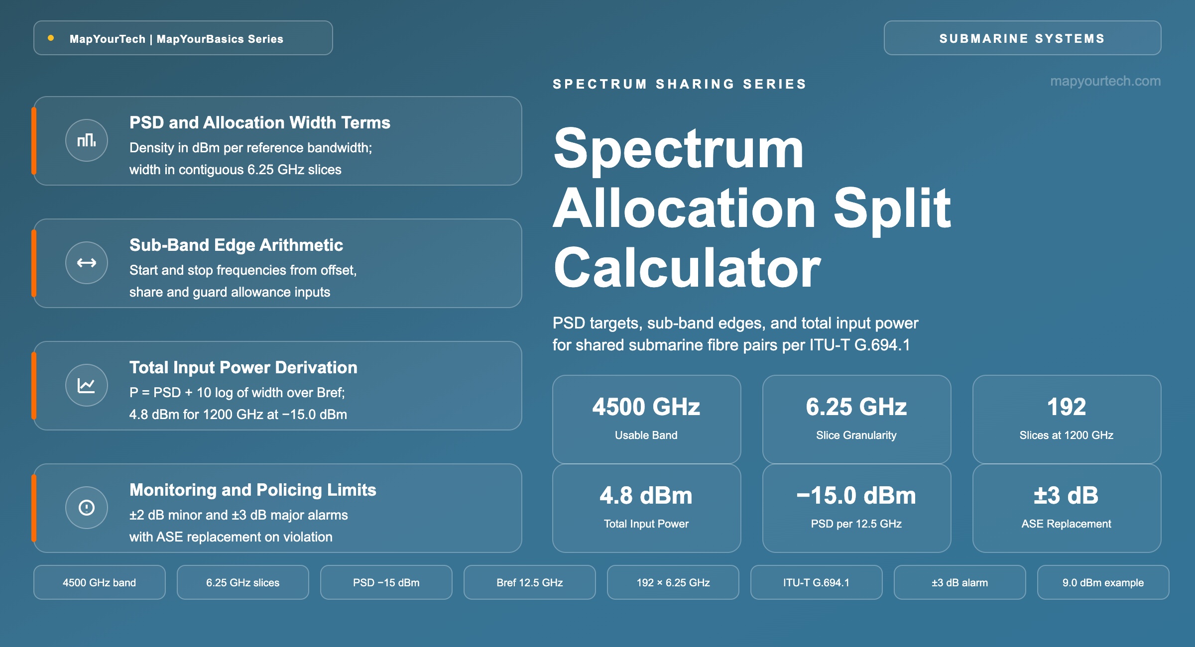
Spectrum Allocation Split Calculator for Shared Fibre Pair
Total available spectrum, requested share and dead-band allowance return the sub-band start and stop frequencies, the allocation width in grid slices, and the total input power implied by the spectral density target at the spectrum user interface.
Guard band is capacity spent on tolerance.
1. Introduction
A shared fibre pair divides its optical spectrum among several spectrum users, each holding one contiguous block behind a spectrum management function that polices frequency range and input power. A typical modern submarine cable system offers 4500 GHz of usable spectrum on one fibre pair, allocated in 6.25 GHz increments (vendor engineering guide; 6.25 GHz is also the flexible-grid granularity that ITU-T G.694.1 specifies), so a 25% share corresponds to 1125 GHz assembled from 180 contiguous slices. The same partitioning logic that governs a submarine allocation also appears in rail-based partitioning of terrestrial line systems, and the wet-plant performance behind each block is specified through the open-cable GSNR framework used in network capacity planning.
The power contract at the spectrum user interface is written twice because the two quantities are measured with different instruments: a power spectral density target requires an optical spectrum analyser to verify, while the total input power derived from that density and the allocation width can be checked with a handheld power meter or a tap-coupler detector during routine monitoring. Because both parties enforce the derived total-power value, the allocation arithmetic — edges, width, slices, and implied power — has to be exact before the contract is signed, in the same way that capacity planning trigger points depend on exact spectrum accounting. This simulator covers that allocation arithmetic at the spectrum user interface; channel engineering inside the allocation, which follows the same DWDM link design parameters as any coherent line, is outside its scope.
2. Power Spectral Density and Allocation Width Definitions
Power spectral density (PSD) at a spectrum user interface is the optical power contained in a fixed reference bandwidth, expressed in dBm per reference slice such as dBm/12.5 GHz. PSD, not total power, is the quantity that sets the gain profile a shared fibre pair presents to every user on it.
Three neighbouring quantities separate as follows. Allocation width is the contracted block between the start and stop frequencies, while usable width is that block minus the dead-band at each edge, where the wavelength selective switch (WSS) filter roll-off leaves too little performance for traffic-carrying channels (working-group definition). PSD is a per-reference-bandwidth quantity, while total power scales with width, so two allocations at the same density but different widths carry different total powers. Slice granularity is the provisioning quantum of the spectrum management hardware, typically 6.25 GHz, while channel spacing is the spectrum user's own plan inside the block and can sit on any grid the allocation accommodates.
The conversion between the two power quantities is one line: Ptotal = PSD + 10·log10(Walloc / Bref), with Ptotal in dBm when PSD is in dBm per reference bandwidth Bref and both widths are in GHz. Worked through for the reference case: a 1200 GHz allocation at a −15.0 dBm/12.5 GHz density target implies −15.0 + 10·log10(96) = −15.0 + 19.8 = 4.8 dBm, about 3.0 mW, at the spectrum user interface (vendor engineering guide worked value, reproduced by this calculator's defaults).
Takeaway: The contract enforces density, but the field verifies power: PSD sets the per-slice level that protects the shared gain profile, and the total-power value derived from PSD and allocation width is what a simple detector checks day to day. Every result below rests on keeping those two quantities, and the width that links them, separate.
3. Allocation Split Calculator
The controls accept the total usable spectrum, the band start frequency, the requested share or width, the placement offset, the dead-band allowance per edge, the slice granularity, and the density target with its reference bandwidth. The result cards return the sub-band edges, the slice count, the dead-band-adjusted usable width, and the implied total input power, with the spectrum map redrawn on every change.
Supports 1000–6100 GHz; 4500 GHz is a typical modern cable (vendor engineering guide)
Low-frequency (red) edge of the shared band; supports 184.000–196.000 THz
Share and width stay synchronized; the engine snaps width to whole slices
Width lost to WSS filter roll-off at each allocation edge; value is vendor-specific
Start frequency f1
192.20000 THz
Band start + offset
Stop frequency f2
193.40000 THz
Start + allocation width
Allocation width
1200.00 GHz
192 slices of 6.25 GHz
Usable width
1175.00 GHz
Dead-band overhead 2.1%
Total input power
4.8 dBm
3.0 mW over the full allocation
Signal power over usable width
4.7 dBm
Same density over traffic-carrying spectrum
4. Total Input Power Versus Allocation Width
Total input power increases by 3 dB for every doubling of allocation width at a fixed density target, because the 10·log10 term is logarithmic in width while the density itself stays constant. The curve below plots the implied power across the full band at the current PSD target and reference bandwidth, with the operating point marking the current allocation; the table beneath it carries the same relation at fixed fractions of the band.
| Case | Width (GHz) | Slices | Power (dBm) | Power (mW) |
|---|
5. Formula Reference
5.1 Sub-Band Edge and Width Relations
Allocation Edges and Slice Count
Walloc = N × g f1 = f0 + Δf f2 = f1 + Walloc Wusable = Walloc − 2 × Wdb
Where: Walloc is the allocation width in GHz; N is the whole number of grid slices; g is the slice granularity in GHz (6.25 GHz standard-specified flexible-grid granularity per ITU-T G.694.1, and the typical provisioning quantum of spectrum management hardware); f0 is the band start frequency in THz; Δf is the placement offset in THz; f1 and f2 are the allocation start and stop frequencies in THz; Wdb is the dead-band allowance per edge in GHz (vendor-specific, set by WSS filter roll-off).
Worked through: a 25% share of a 4500 GHz band requests 1125 GHz, which is exactly 180 slices at 6.25 GHz granularity, so no snapping is needed (vendor engineering guide example). Placed at zero offset on a band starting at 191.300 THz, the allocation runs from 191.300 to 192.425 THz, and a 12.5 GHz dead-band at each edge leaves 1100 GHz of traffic-carrying spectrum.
5.2 Total Input Power From Spectral Density
Density-to-Power Conversion
Ptotal = PSD + 10·log10(Walloc / Bref)
Where: Ptotal is the total input power at the spectrum user interface in dBm; PSD is the density target in dBm per reference bandwidth (typical contract values sit near −15.0 dBm/12.5 GHz or −10.0 dBm/6.25 GHz, working-group and vendor example parameters); Walloc is the allocation width in GHz; Bref is the PSD reference bandwidth in GHz, agreed per contract because it is vendor-specific.
Worked through: at −15.0 dBm/12.5 GHz over 1200 GHz, the ratio Walloc/Bref is 96, its logarithmic term is 19.8 dB, and the implied total input power is 4.8 dBm (vendor engineering guide worked value). The same arithmetic run backwards recovers a width from a power target: a 9.0 dBm total at −10.0 dBm/6.25 GHz implies 101.9 × 6.25 ≈ 496 GHz, which snaps down to 79 slices, or 493.75 GHz (working-group example parameters).
6. Practical Example
Practical Example — 1200 GHz allocation on a 4500 GHz shared fibre pair
A spectrum user requests 1200 GHz on a fibre pair with 4500 GHz of usable spectrum starting at 191.300 THz, a 26.7% share assembled from 192 contiguous 6.25 GHz slices. The fibre pair owner places the block 900 GHz above the band start, so the contracted edges are 192.200 and 193.400 THz. A 12.5 GHz dead-band at each edge, set by the WSS filter roll-off of the spectrum management hardware, subtracts 25 GHz and leaves 1175 GHz of traffic-carrying spectrum, a 2.1% overhead. At the contracted density target of −15.0 dBm/12.5 GHz, the derived total input power is 4.8 dBm, about 3.0 mW, and that single dBm figure becomes the value a tap-coupler detector polices during operation (vendor engineering guide worked value). These defaults are pre-loaded in the calculator above, so every number in this paragraph is reproduced on screen.
7. Monitoring and Policing Considerations
The derived total-power value carries alarm thresholds on both sides: working-group example contract parameters place a minor alarm at ±2 dB and a major alarm with automatic ASE replacement at ±3 dB from the agreed input power, with a configurable hold-off before the spectrum management function substitutes amplified spontaneous emission for an invalid input (working-group example values). ASE replacement exists because a missing or over-powered allocation changes the gain profile of the shared amplifier chain for every other user, the same coupling that makes fiber bandwidth and capacity engineering a whole-band exercise rather than a per-channel one.
A density violation can occur even when the total power is compliant, because power concentrated into part of the allocation raises the local density while the aggregate stays inside its thresholds; routine total-power monitoring therefore complements, and does not replace, periodic optical spectrum analyser sweeps. On dispersion-compensated legacy cables, ASE loading behaves less benignly than on uncompensated D+ cables, so wider dead-bands and additional traffic engineering rules apply and the allocation arithmetic above starts from a smaller effective band (vendor engineering guide). The receive side of the same interface applies the reference-bandwidth discipline familiar from OSNR reference-bandwidth conversion in coherent DCI links: a density quoted without its reference bandwidth is not a specification.
8. Summary
A spectrum sharing contract reduces to five numbers per allocation: two edge frequencies, one width in whole grid slices, one density target with its reference bandwidth, and one derived total input power. The width follows from the requested share and the granularity, the edges follow from the band start and the placement offset, the usable width subtracts the dead-band at each edge, and the power follows from the density through a single logarithmic term. Holding those relations exact at contract time is what lets a handheld power meter enforce, for the life of the service, a specification that only an optical spectrum analyser can fully characterize.
9. References
- SubOptic Spectrum Sharing Working Group — Spectrum Sharing White Paper, SubOptic Association.
- Ciena — The Spectrum Sharing Handbook, Ciena.
- ITU-T G.694.1 — Spectral grids for WDM applications: DWDM frequency grid, ITU-T Study Group 15.
Related Articles on MapYourTech