
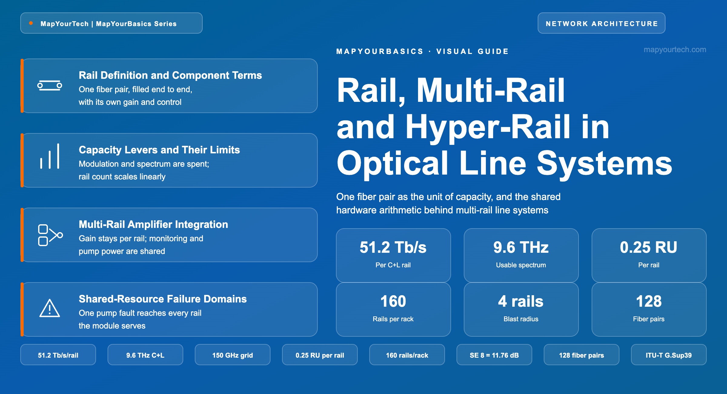
Rail, Multi-Rail and Hyper-Rail in Optical Line Systems
A visual guide to the fiber pair as the unit of optical capacity, the shared-hardware arithmetic that makes multi-rail amplification possible, and the correlated failure modes that come with it.
Spectrum is the one asset a network cannot manufacture more of.
What You Will Learn
- What a rail is, what it contains, and how it differs from a wavelength, a fiber pair and a line system
- What drives rail-based scaling: the collective traffic of distributed training, and fibers filling for everyone else
- Why two of the three capacity levers are close to exhausted, with the SNR and reach arithmetic behind that
- Why the word "rail" means one thing in a GPU back-end fabric and another in an optical line system
- How a multi-rail in-line amplifier shares monitoring, equalization and pump power across four or more fiber pairs
- The rack-unit and power arithmetic that turns 8 RU of amplification into 1 RU
- Which failure domains widen when hardware is shared, and how to place protected pairs against that
- What the four vendors that announced multi-rail products in 2026 have each specified
1. Introduction
An in-line amplifier hut on a long-haul route holds a fixed number of racks, draws a fixed power feed, and runs a cooling plant sized when the building was commissioned. None of that changes when the traffic between two data centers grows from four fiber pairs to two hundred. A hyperscale operator presented at OFC 2026 that regional data center interconnection has typically needed 16 to 48 fiber pairs, while AI-driven regional interconnection needs 128 or more (operator statement). Amplifying 128 fiber pairs with one conventional line system per pair places roughly six racks of amplifier equipment into a building with floor space and power for two.
That arithmetic produced the rail. For three decades the unit of capacity growth in optical transport was the wavelength: fill the C-band one channel at a time, extend into the L-band, then raise the baud rate. The rail moves the unit up one level, to the whole fiber pair, and the growth step becomes a rail rather than a channel. Once the step size changes, the equipment changes with it, because a line system built to serve one fiber pair per chassis cannot serve two hundred of them inside an existing building.
Four major optical suppliers put multi-rail products into the public record during 2026, and three more were reported to be evaluating systems of their own, with commercial shipments assessed as likely to begin during 2027 (analyst assessment). One of the four markets its platform under the hyper-rail name and states that hyper-rail is sometimes called multi-rail; analyst and trade coverage has settled on multi-rail as the generic term, and this guide follows that usage. Suppliers appear below as Vendor A through Vendor D, and each label means the same supplier in every section and figure.
The sections below define the rail from first principles, separate it from the three terms it gets confused with, work the density and power arithmetic, and state the conditions under which the architecture stops paying. The application context is scale-across data center interconnection, where coherent links tie accelerator clusters in separate buildings into one training fabric.
2. Rail Definition and Component Terms
A rail is one fiber pair carrying a fully filled optical spectrum end to end, together with the amplification, monitoring and control that keep it in specification. A rail is counted, not measured: capacity grows by adding rails rather than by adding wavelengths to a fiber that is already full.
Two properties in that definition carry the weight. The first is fully filled. A fiber pair carrying eight of sixty-four possible channels is a partly used fiber pair, and its remaining capacity costs nothing but a transponder; a rail is the unit an operator reaches for once that headroom is gone. The second is instrumented as one managed unit. A rail holds its own gain targets, its own tilt correction, its own optical supervisory channel (OSC) identity and its own alarm set, which is what allows a hundred rails to run over one route without collapsing into an undifferentiated bundle of glass.
2.1 Distinctions From the Adjacent Terms
A rail is not a wavelength. A wavelength is one carrier occupying one frequency slot inside a rail's spectrum, so a single C+L rail on a 150 GHz grid holds 64 of them.
A rail is not simply a fiber pair. Every rail is a fiber pair, but a dark or partly lit pair becomes a rail only when it is filled, amplified and instrumented as a managed unit, which is why rail counts and fiber counts diverge on routes with spare glass in the ground.
A rail is not a line system. The line system is the equipment chain — terminals, amplifiers, equalizers, supervisory channels — and a multi-rail line system serves several rails from one set of shared modules.
A rail in an optical line system is not a rail in a back-end fabric. Inside the data center, a rail names the set of like-indexed accelerator ports homed to one leaf switch; between data centers it names a fiber pair, and Section 3 separates the two.
2.2 Units and Conversion Arithmetic
Crail = ( B / Δf ) × Rch
Where:
- Crail — capacity of one rail in one direction, in b/s. Typical range today: 25–80 Tb/s.
- B — usable optical spectrum per fiber, in Hz. Typical range: 4.8 THz for C-band alone, 9.6 THz for C+L.
- Δf — channel spacing, in Hz. Typical range: 75–225 GHz, set by the symbol rate and roll-off of the carrier.
- Rch — per-channel line rate, in b/s. Typical range: 400 Gb/s to 1.2 Tb/s.
Practical Example — capacity of one C+L rail carrying 800G channels
Take a C+L line system with 9.6 THz of usable spectrum across the two bands, carrying 800 Gb/s coherent channels on a 150 GHz grid. The channel count is 9.6 THz ÷ 150 GHz = 64 carriers per direction, and the rail capacity is 64 × 800 Gb/s = 51.2 Tb/s. Vendor A states the same 9.6 THz and 51.2 Tb/s figures for its C+L multi-rail platform with 800G transceivers, rising to 76.4 Tb/s with 1.2 Tb/s embedded engines (vendor claim, Vendor A). Swap the transceiver and the rail capacity changes; run out of spectrum and only a second rail moves the number.
Takeaway: the rail is a countable unit of filled, instrumented fiber capacity. Everything that follows — the density arithmetic, the shared-hardware design and the widened failure domains — comes from treating that unit, rather than the wavelength, as the thing an operator adds.
3. Rail Terminology Across Compute and Transport Layers
The word arrives in optical engineering already carrying a different meaning from the compute side, and the two definitions sit two layers apart in the same AI network. Inside the data center, a rail-optimized back-end fabric homes accelerator port 0 on every server to leaf switch 0, port 1 to leaf 1, and so on; each of those port-to-leaf groupings is a rail, and the design exists so that collective operations between like-indexed accelerators stay one hop from each other. Between data centers, a rail is a fiber pair. Neither usage is wrong, and both appear in the same architecture review.
The practical consequence appears whenever a number is quoted without its layer. "We run 128 rails" describes a fabric topology if the speaker works on the switching side and 128 fiber pairs of coherent transport if the speaker works on the optical side, and the two numbers have no fixed relationship to each other. The optical rail count follows from the aggregate inter-site bandwidth divided by the capacity of one rail; the fabric rail count follows from the number of accelerators per server. Ask which layer before designing against the figure.
Scale-across sits between the two. It names the case where accelerator clusters in separate buildings are joined tightly enough to run one training job, which is a compute requirement met with optical hardware. Neocloud operators and hyperscalers arrive at the same conclusion from different directions: power and floor space run out at one site before the compute requirement does, so the fabric extends over fiber, and the fiber count follows the fabric bandwidth.
Takeaway: a rail count is meaningless without its layer. On the optical side it counts fiber pairs; on the fabric side it counts port-to-leaf groupings, and the two are set by unrelated design rules.
4. Traffic Drivers for Rail-Based Scaling
A distributed training job generates a traffic pattern that data center interconnection was not sized for. On every training step, each participating accelerator exchanges gradient values with its peers so that all copies of the model converge on the same parameters, and the step does not complete until that exchange completes. The link therefore runs close to line rate for the duration of the exchange rather than averaging out over a daily cycle, and the figure that governs the design is the time to complete the collective operation rather than mean throughput. Traffic of this shape rewards capacity and punishes congestion, and it does so on every step of a run that may last weeks.
The reason that exchange crosses fiber at all is electrical and civil rather than optical. A site has a fixed power feed and a fixed floor area, and both cap the number of accelerators it can hold. When the training requirement exceeds what one site can power, the cluster is split across buildings, campuses and increasingly across regions to reach available power and real estate, and the fabric that joined accelerators inside one hall has to cross tens or hundreds of kilometres instead. Vendor B describes clusters scaling from thousands to millions of accelerators and becoming geographically distributed for exactly that reason, with the resulting interconnect requirement reaching tens of petabits per second across hundreds of fiber pairs (vendor statement, Vendor B).
Two numbers set the scale of the change. A hyperscale operator presented at OFC 2026 that regional data center interconnection has typically needed 16 to 48 fiber pairs, while AI-driven regional interconnection needs 128 or more (operator statement). That is not a percentage increase on an existing design; it is a different order of quantity arriving at buildings whose rack count and power feed were fixed years earlier. The wider architectural consequences reach the transponder and router layers as well, and the amplifier sites feel them first, because those are the places on the route where equipment has to sit and where nobody planned for a fourfold increase in it.
A second driver runs alongside the first and receives less attention. Operators with no AI workload at all arrive at the same conclusion by a different route, because their fibers are also filling. Vendor A describes service providers, wholesale carriers and neocloud operators looking to grow in the shadow of the Shannon limit, and reaching multi-rail deployment in conventional data center interconnection and managed optical fiber network applications as a consequence (vendor statement, Vendor A). Once a route's existing pairs are full and the spectral efficiency lever has stopped delivering, adding pairs is what remains, whatever the traffic on them happens to be.
Size the rail count against the aggregate inter-site bandwidth at end of life, then divide by the capacity of one filled pair. A design sized against first-year traffic will be correct for a year and will then send engineers back to the amplifier sites, which is the one part of the route where a revisit means civil work rather than a card swap.
Takeaway: the driver is a compute placement decision rather than an optical one. Power and floor space cap the accelerators at a site, the job spans sites in response, and the collective exchange between them converts directly into fiber pairs on a route.
5. Wavelength Scaling and Its Capacity Ceiling
Three levers add capacity to a route: carry more bits in each symbol, occupy more optical spectrum, or light more fiber pairs. The first two were the levers of the previous three decades, and both are now close to their limits for reasons that are separate and worth stating with numbers, because the phrase "approaching the Shannon limit" is used loosely enough that it no longer conveys how little headroom remains.
5.1 Modulation Order and the Reach Penalty
Capacity on a channel limited by additive Gaussian noise follows Shannon's relationship, which takes this form for a dual-polarization coherent carrier.
C = 2 · B · log2(1 + SNR) SNR = 2(SE/2) − 1
Where:
- C — channel capacity in b/s. The factor 2 counts the two polarizations.
- B — symbol rate in Bd, which is also the noise bandwidth of a matched receiver.
- SNR — signal-to-noise ratio in the symbol-rate bandwidth, as a linear ratio.
- SE — spectral efficiency C/B in b/s/Hz for the dual-polarization carrier. Typical deployed range: 4–12 b/s/Hz.
Inverting the relationship is what exposes the ceiling. Reaching a spectral efficiency of 8 b/s/Hz requires a linear signal-to-noise ratio of 15, which is 11.76 dB; reaching 10 b/s/Hz requires 31, which is 14.91 dB. One additional bit per second per hertz therefore costs a little over 1.5 dB of signal-to-noise ratio at the efficiencies deployed systems operate at, and that cost rises with every further step because the relationship is exponential in spectral efficiency.
| Representative format | SE (b/s/Hz) | Required SNR (dB) | Relative reach |
|---|---|---|---|
| DP-QPSK | 4 | 4.77 | 1.00 |
| Shaped, between QPSK and 16QAM | 6 | 8.45 | 0.43 |
| DP-16QAM | 8 | 11.76 | 0.20 |
| Shaped, between 16QAM and 64QAM | 10 | 14.91 | 0.10 |
| DP-64QAM | 12 | 17.99 | 0.05 |
Two qualifications belong with that table, and both make the picture worse rather than better. The SNR column is the Gaussian bound (theoretical limit): a deployed modulation format with real forward error correction needs several decibels more than the bound to reach the same spectral efficiency, so the practical curve sits to the right of these values. The relative reach column assumes amplified spontaneous emission is the only noise source, so that optical signal-to-noise ratio falls in proportion to the number of spans and reach scales as the inverse of the required linear SNR. Nonlinear interference does not behave that way, since it grows with launch power and cannot be outrun by turning the transmitter up, and including it shortens the high-efficiency rows further.
The engineering consequence is what the table makes visible. Moving from 16QAM at 8 b/s/Hz to 64QAM at 12 b/s/Hz is a 50% capacity gain that costs roughly three quarters of the reach even in the ideal case. That trade is worth taking on an 80 km data center interconnect span and is unavailable on a 700 km route, which is why long-haul designs settled around QPSK and shaped formats between QPSK and 16QAM rather than climbing the constellation ladder. The lever still moves; it moves a short distance for a large price.
5.2 Symbol Rate as a Separate Question
Raising the symbol rate is often described as a fourth capacity lever, and at the level of the fiber it is not one. Capacity per fiber is the usable spectrum multiplied by the spectral efficiency achieved in it, so a 200 GBd carrier occupying 225 GHz and a 100 GBd carrier occupying 112.5 GHz deliver the same total across the band at the same spectral efficiency — the higher-baud system uses fewer, wider channels to get there. What the higher symbol rate does buy is real and lies elsewhere: fewer transponders, fewer client ports, and lower cost and power per bit, since one high-baud modem replaces two lower-baud ones. Those are the economics of the terminal rather than the capacity of the glass.
A supplier quoting a higher per-wavelength rate is quoting a transponder capability. Whether route capacity rises with it depends on whether spectral efficiency rose too. An 800 Gb/s carrier in 150 GHz and a 400 Gb/s carrier in 75 GHz occupy the same band to the same effect.
5.3 Optical Bandwidth and the Erbium Boundary
The second lever was spectrum, and it delivered one doubling. ITU-T G.Sup39 places the conventional C-band at 1530 to 1565 nm and the long-wavelength L-band at 1565 to 1625 nm (standard-specified). No commercial system uses the full L-band definition, because the erbium gain coefficient falls below usable levels well before 1625 nm and practical L-band amplifiers cover roughly 1570 to 1610 nm, so a deployed C+L line system operates with close to 4.8 THz per band and about 9.6 THz in total.
Adding the second band returns less than a clean factor of two, for four reasons that all appear in the link budget. Stimulated Raman scattering transfers power from the shorter wavelengths to the longer ones across the occupied spectrum, producing a tilt reported at up to about 8 dB per span at full fill on standard single-mode fiber (measured, industry practice), which the amplifier chain corrects span after span. The L-band amplifier noise figure runs roughly 1 dB worse than its C-band counterpart. Band splitters and combiners add insertion loss at every amplifier and every node. And fiber attenuation rises toward the long-wavelength end of the band. The migration from C-band to C+L is a well-established operation and the capacity it returns is real, but the lever is single-use: once both bands are lit, there is no third erbium band behind them.
Bands beyond C+L need a different amplification technology rather than a different filter — a different dopant, or distributed Raman amplification across the new band — and none of those is in volume production on terrestrial line systems. Treat additional bands as a research and early-trial subject rather than as a capacity option available to a route being designed now.
5.4 Rail Count and What Bounds It
The third lever behaves differently from the other two, and the difference is what makes it the one in use. Capacity per rail stays constant as rails are added, so route capacity scales linearly with rail count, and the per-rail optical design — launch power, span loss, tilt correction, spectral efficiency — is unchanged from the single-rail case the engineering team already knows how to close. Adding a rail adds no impairment to the rails beside it, because each pair carries its own light in its own glass. That is a rare property: the first two levers degrade the quantity they improve, and this one does not.
What bounds it is not physics. Rail count is limited by fiber pairs available in the ground, by rack space at the amplifier sites, and by the power and cooling those buildings can supply — constraints that are commercial, civil and negotiable in a way the Shannon bound is not. The arithmetic in Figure 4 sets the scale: a route carrying 6.5 Pb/s in aggregate needs 127 rails at 51.2 Tb/s per rail, and raising the per-channel rate to 1.2 Tb/s reduces that to about 86 — a useful reduction that leaves the rail count in three figures. No plausible transponder generation returns the route to a single fiber pair, which is why the equipment question moved from the transponder to the line system.
Takeaway: modulation costs about 1.5 dB of required SNR per additional b/s/Hz and pays for it in reach; spectrum delivered one doubling and has no third erbium band behind it; rail count scales linearly and is bounded by buildings. When the binding constraint moves from physics to buildings, the engineering response moves to integration density.
6. Single-Rail In-Line Amplifier Inventory
A conventional C+L in-line amplifier shelf serves exactly one fiber pair, and it carries a complete set of hardware to do so. The incoming spectrum meets a C/L splitter, the two bands are amplified in separate erbium-doped fiber amplifiers because the erbium gain spectrum has a deep dip between them, each band passes a dynamic gain equalizer to correct the tilt and ripple accumulated over the preceding spans, and a combiner returns them to one fiber. The west direction repeats the chain. Around that optical path sit an optical channel monitor, an optical supervisory channel transceiver, an optical time-domain reflectometer, a control processor, power supplies and fans.
The design is correct and has been for two decades. Its property that becomes a problem at scale is that every block belongs to one fiber pair. The optical channel monitor watches one spectrum, the reflectometer tests one fiber, the control processor manages one amplifier chain, and the fans cool one shelf. Nothing in the shelf is available to the pair in the next rack, so the hardware count grows exactly in proportion to the rail count.
Suppliers state around 8 RU in a 300 mm design for four C+L in-line amplifiers, which is 2 RU per rail (vendor data). A 40 RU rack therefore holds 20 rails, and 128 rails need 6.4 racks of amplification at every in-line site along the route. On a 700 km route with amplifier huts at roughly 85 km spacing there are about eight such sites, so the same 128 rails need in the order of 51 racks of amplifier equipment between the two terminals — before any terminal, transponder or add/drop hardware is counted.
Takeaway: the conventional shelf is not inefficient at what it does; it is dedicated. Dedication is affordable at four rails and unaffordable at 128, and the monitoring and housekeeping functions are where the duplication concentrates.
7. Multi-Rail Amplifier Integration
A multi-rail amplifier card keeps the gain stages per rail and shares everything that can be shared. Gain cannot be pooled, because gain is a property of one fiber carrying one set of channels over one span loss: the amplifier for rail 3 has to hit rail 3's target output power with rail 3's tilt correction, and no averaging across rails produces that. Monitoring, supervisory signalling, reflectometry, equalization control, pump power and housekeeping are a different case. Each of those either measures one rail at a time, which allows time-multiplexing, or supplies energy that can be divided among several gain stages.
Vendor A describes its multi-rail card as supporting four fiber rails in 1 RU with shared dynamic gain equalization, optical channel monitoring, supervisory channel and reflectometry across the rails, and states that power per rail falls by more than 60% through the integration (vendor claim, Vendor A). Vendor D describes four C+L transport rails within a single 1 RU in-line amplifier card (vendor claim, Vendor D). The two descriptions agree on the mechanism even where the platforms differ, which is a fair indication that the four-rails-per-RU figure reflects what the components currently allow rather than one supplier's packaging choice.
| Function | Allocation | Reason |
|---|---|---|
| C-band and L-band gain stages | Per rail | Output power and tilt targets are properties of one fiber and one span loss |
| Band splitter and combiner | Per rail | Sits in the optical path of a single fiber |
| Gain, power and tilt setpoints | Per rail | Each rail closes its own link budget and reports its own OSNR |
| Optical channel monitor | Shared, time-multiplexed | A spectrum sweep takes milliseconds, so one monitor can visit several ports in sequence |
| Optical supervisory channel | Shared with per-rail identity | One transceiver assembly carries the management path; each rail keeps its own address |
| Optical time-domain reflectometer | Shared, switched | Fiber characterization runs on demand rather than continuously |
| Equalization control | Shared processing, per-rail profiles | The equalization profile is computed per rail but executed by common logic |
| Pump lasers | Shared, multi-chip | Uncooled multi-chip pump assemblies feed several gain stages from one package |
| Control processor, power, cooling | Shared | Housekeeping load per rail falls as the card carries more rails |
The pump laser row carries most of the power saving and most of the risk. Removing the thermoelectric cooler from a pump laser and packaging several pump chips in one assembly is what lets one card feed eight gain stages within a 1 RU power envelope, and two of the four suppliers name uncooled or multi-chip pumps as the enabling component. It also means one pump assembly now sits in the path of four rails, which Section 9 treats. Supply is the second consideration: uncooled multi-chip pump lasers come from a small number of manufacturers, so pump availability rather than card design sets how fast a multi-rail deployment can proceed.
Terminal equipment is following the same integration path. Vendor A's terminal module places C-band and L-band pre-amplifiers and boosters, a twin C+L 1×66 wavelength selective switch, amplified spontaneous emission loading, supervisory channel, channel monitor and reflectometer into a 2 RU module (vendor claim, Vendor A). ASE loading is worth noting for anyone turning up rails in stages: it fills unused spectrum with shaped noise so that the amplifier chain sees a constant total load, which keeps per-channel performance the same on day one as at full fill and removes a whole class of re-optimization work from the turn-up of rail number ninety. The band allocation decision and the tilt and ripple management for each rail are unchanged from the single-rail case.
Verify that the shared optical channel monitor's revisit interval across all rails on a card is short enough for the control loop that depends on it. A monitor serving four rails samples each one a quarter as often as a dedicated monitor, which is acceptable for equalization but changes the detection latency for a fast power transient.
Takeaway: the split is clean and physical. Anything that carries or shapes one fiber's light stays per rail; anything that measures, signals, computes or supplies energy can be shared, and that is where the space and power come from.
8. Rail Density and Power Arithmetic
Two stated footprints set the density step. Four C+L in-line amplifiers occupy about 8 RU in current 300 mm designs, and a multi-rail card carries four rails in 1 RU (both vendor data). That is 2 RU per rail against 0.25 RU per rail, so a 40 RU rack holds 20 rails in the conventional design and 160 in the multi-rail design — an eight-fold step derived from the two published footprints.
| Quantity | Conventional | Multi-rail | Evidence class |
|---|---|---|---|
| Rack units per four C+L rails | 8 | 1 | Vendor-stated footprint |
| Rack units per rail | 2.00 | 0.25 | Derived from the row above |
| Rails per 40 RU rack | 20 | 160 | Derived |
| Racks needed for 128 rails, one site | 6.4 | 0.8 | Derived |
| Power per rail, index | 100 | <40 | Vendor claim, more than 60% reduction |
Headline multipliers in supplier material sit above the eight-fold figure derived here, because each supplier picks its own baseline. Vendor A states a 40-fold increase in in-line amplifier density and describes traditional designs needing 12 RU or more for the same four rails; Vendor B states up to 32 times density improvement and 75% power savings for its hyper-rail platform (both vendor claims). A 12 RU baseline gives about 13 rails per rack and a twelve-fold step; a 40-fold ratio implies a baseline of four rails per rack, which corresponds to a different equipment generation than the 8 RU figure. None of the numbers is wrong — they answer different questions — and the design consequence is to work the arithmetic against the footprint of the equipment installed at the site in question rather than against a published ratio.
Practical Example — amplifier footprint on a 700 km route carrying 128 rails
Take a 700 km point-to-point route with in-line amplifier huts at roughly 85 km spacing, giving eight in-line sites, and a target of 128 filled fiber pairs. In the conventional design, each site needs 128 × 2 RU = 256 RU, which is 6.4 racks, and the route needs about 51 racks of in-line amplification in total. With four rails per RU, each site needs 128 × 0.25 RU = 32 RU, which is 0.8 of a rack, and the route needs about 6.4 racks. The route-level difference is around 45 racks of equipment, distributed across eight buildings that were never designed to hold it — which is the reason the first multi-rail orders came from operators with existing huts rather than from greenfield builds.
Power follows the same shape but with a different mechanism. Housekeeping load — control processor, fans, power conversion, monitoring — is close to fixed per shelf, so spreading it across four rails divides it by four, while the gain stages themselves still consume pump power in proportion to the optical power they deliver. That is why the stated saving is a per-rail figure of more than 60% rather than a total-power figure: the fraction that scales with traffic does not disappear, and the fraction that scales with shelf count does. On a site where the power feed is the binding constraint, the useful question is how many rails the available kilowatts support, not what percentage the supplier quotes.
Takeaway: derive the density step from the two footprints that apply to your site, not from a published multiplier. The reliable arithmetic is rack units per rail and watts per rail, and both are available from any supplier that quotes a card.
9. Shared-Resource Failure Domains
Sharing a pump assembly across four rails creates a failure mode that per-rail systems do not have. In a conventional site, a pump failure removes the rail whose shelf it sits in and leaves the other rails at that site untouched, so the fault domain and the traffic domain are the same size. On a multi-rail card, the same failure degrades the gain of every rail the pump feeds, and the four rails fail together whether or not they carry related traffic. The same applies to the shared control processor, the shared power conversion and the shared cooling path.
This is a placement problem, not an availability objection. Optical networks have always carried correlated failure domains — a duct cut takes every fiber in the duct, a cable landing takes every pair in the cable — and the discipline for handling them is established: identify the shared risk, record it, and place the two halves of any protected pair on different instances of it. Multi-rail adds card, shelf and pump assembly to the list of things a shared-risk group has to name, alongside duct, cable, conduit and building.
Four practical consequences follow. Protected pairs go on different cards and different shelves, never on two rails of one module, which costs nothing if it is decided during rail assignment and is expensive to correct afterwards. Shared-risk group data needs the module-level identifiers, which means the inventory system has to carry them and the path computation has to read them. Per-rail telemetry has to be retained even where the measuring instrument is shared, because an operator seeing four rails degrade at once needs to distinguish a shared-pump fault from four coincident fiber events. And the maintenance procedure for replacing one card has to be established before the first replacement rather than during it: whether the card can be swapped without interrupting the other rails it carries determines whether the maintenance window is minutes of one rail or hours of four.
Sharing a component does not raise its failure rate, and the change that always occurs is the traffic reached by one failure. Whether per-rail availability itself changes depends on what the sharing does to each rail's series component count. Where a shared controller, power converter or cooling path replaces a dedicated one roughly one for one, the count is unchanged and per-rail figures carry across; where sharing inserts additional elements into the optical path, such as a splitter network distributing one pump across several gain stages, those elements enter every rail's availability model and have to be added to it. Rebuild the model with the common-resource elements and their redundancy explicitly in it, and recompute expected traffic loss per event separately, before quoting a service level on a multi-rail route.
Takeaway: the failure domain widens from one rail to the group a module serves. Extend the shared-risk group model to card and pump identity, keep per-rail telemetry, and place protected pairs across modules before the rails are assigned.
10. Multi-Rail Platform Specifications
Four major optical suppliers put multi-rail products into the public record during 2026, and their published specifications differ in what they disclose rather than in the mechanism they describe. Vendor A and Vendor D both state four C+L rails in a 1 RU in-line amplifier card. Vendor C states up to 128 fiber pairs per rack for its multi-rail open line system. Vendor B states a density and power ratio against its own previous generation rather than a rails-per-rack-unit figure. Every number in the table below is a supplier statement, none has been independently measured in a published field trial, and the vendor labels are the same ones used in every other section of this guide.
| Supplier | Stated integration | Stated density and power | Stated availability |
|---|---|---|---|
| Vendor A | Four C+L rails per 1 RU, with shared equalization, channel monitoring, supervisory channel and reflectometry | Up to 160 rails in a 40 RU 600 mm rack; power per rail lower by more than 60% | Second half of 2026 |
| Vendor B | Multiple fiber pairs in parallel over hundreds of kilometres; 300 mm and 600 mm variants | Up to 32 times density improvement and 75% power savings against its own previous line system | First multi-rail order awarded during 2026; deployments rolling out through 2027 |
| Vendor C | Multiple fibers into one amplifier; uncooled multi-pump chips and multi-rail equalizers | Up to 128 fiber pairs per rack | Announced during 2026; availability not publicly stated |
| Vendor D | Four C+L transport rails within a single 1 RU in-line amplifier card | Density figure not publicly stated | Demonstrated with 800G ZR transceivers during 2026 |
Three further suppliers were reported to be evaluating multi-rail systems of their own, with commercial shipments of multi-rail products assessed as likely to begin during 2027 (analyst assessment). That timing constrains procurement: a route being designed now will be built with equipment that is still pre-shipment for most of the supply base, so a design that assumes multi-rail amplification needs a conventional fallback for the sites that have to be turned up first. For the component-level view of how the same integration pressure reshaped terminal and transponder hardware, the MapYourTech treatment of compact modular optical hardware covers the preceding two generations, and the multi-rail line system analysis works the integration progression in more depth than a visual guide allows.
Supplier statements in this guide carry a label rather than a company name, and each label means the same supplier in every section, table and figure. Every such statement is marked with its evidence class in the sentence that contains it — vendor claim, vendor statement, vendor data, operator statement or analyst assessment — so a reader can separate what a supplier asserts from what this guide derives. Derived quantities are marked as derived in Table 3 and are reproducible from the two footprints above them. The References list holds the standards and public documents the physics and grid arithmetic rest on; supplier product statements are not standards documents and are not listed there.
Takeaway: the disclosed specifications agree on four rails per rack unit where they state a figure at all, and disagree on headline ratios because each baseline differs. Procurement timing, not architecture, is the open question through 2027.
11. Applicability Conditions and Design Limits
Four conditions decide whether multi-rail amplification pays on a given route, and a negative answer to any of them points back to a conventional design. The first is rail count. At low rail counts, conventional amplification often remains the economic choice, because the shared functions have too little traffic to amortise; the break-even point is specific to the platform, the site and the commercial model, and around 16 filled fiber pairs serves as an illustrative planning threshold rather than a specified limit. The second is site constraint: where rack space and power at the in-line sites are available, the density gain buys nothing that the operator needs. The third is route homogeneity: rails sharing one card should share a route and a span plan, since a card serving two different span-loss profiles will run some of its gain stages away from their design point. The fourth is node type, because a multi-degree add/drop node needs per-rail switching flexibility that a shared, high-density amplifier card is not built to provide.
Mixed designs are normal and worth planning for. A route can run multi-rail amplification between two terminals and conventional router-attached or ROADM equipment at its ends, because the constraint that multi-rail relieves lives at the in-line sites rather than at the terminals. Equally, a route may carry 128 rails between two campuses and four rails on a spur, and there is no reason for both segments to use the same amplifier generation.
Two limits deserve stating plainly. Multi-rail integration does not change per-rail optical performance, so a route that fails its optical signal-to-noise ratio budget with conventional amplification fails it with multi-rail amplification as well; the technology addresses space and power, not reach. And rail count is bounded by fiber in the ground. An operator with 48 pairs on a route cannot run 128 rails regardless of amplifier density, which puts duct and cable acquisition — not equipment selection — on the critical path for the largest scale-across builds.
Takeaway: multi-rail addresses space and power at in-line sites. It leaves reach, spectral efficiency and fiber availability exactly where they were, and a route that is short of any of those three needs a different answer.
12. Amplifier Site Power and Cooling
Denser amplification moves the constraint from rack space to heat. Vendor B states that in some cases as much as 70% of amplifier site power is consumed by cooling equipment, and that hut designs have to change — airflow, cooling efficiency and supported power per rack — before higher rail counts per site can be realised (vendor statement, Vendor B). The arithmetic is direct: a rack drawing four times the power in the same floor area rejects four times the heat into a building whose cooling plant was sized for the equipment generation it was built around.
Rack depth appears in the specifications for the same reason. Vendor A's highest-density configuration quotes 160 rails in a 40 RU rack at 600 mm depth, against conventional four-rail amplifiers in 300 mm shelves, and Vendor B offers both 300 mm and 600 mm variants of its platform (vendor data). The extra depth is airflow path and heat-sink volume, and it is a real deployment constraint in older huts built for 300 mm equipment where cabinet depth, not rack units, is what runs out first.
Three site-level checks belong in the survey before a multi-rail design is committed. Confirm the available power feed per rack position and compare it against the card's stated draw at full rail load, not at the shipping configuration. Confirm the cooling capacity and the inlet temperature at the top of the rack, since a fully populated multi-rail rack concentrates heat that a partly filled conventional rack spread across several cabinets. And confirm cabinet depth and cable management, because 160 rails means 320 fibers entering one rack, and fiber routing at that density becomes a physical design task in its own right.
Turning up rails in stages keeps per-rail performance constant only if unused spectrum is loaded. Amplified spontaneous emission loading fills the empty slots with shaped noise so the amplifier chain sees a constant total input power, which is what allows rail 90 to be added without re-optimising rails 1 to 89. Confirm the loading behaviour of the platform before planning a staged fill.
Takeaway: the density is available before the buildings are ready for it. Power feed per rack, cooling capacity at the top of the rack, and cabinet depth are the three site figures that decide how many rails a given hut can hold.
13. Conclusion
The rail is a unit of accounting that follows from a physical fact: the spectrum in one fiber is finite, coherent transponders already work close to its information-theoretic ceiling, and inter-site bandwidth requirements now exceed what one fiber pair can carry by two orders of magnitude. Once capacity is added a fiber pair at a time, the equipment that amplifies fiber pairs has to be counted differently, and the four platforms in the public record all answer that by sharing monitoring, equalization control, pump power and housekeeping across four or more rails while keeping gain per rail.
Three figures carry the engineering content of the change. Rack units per rail falls from about 2.00 to 0.25 on stated footprints, which turns 6.4 racks of amplification per site into 0.8. Power per rail falls by a stated 60% or more, concentrated in the housekeeping load rather than in the pump power that scales with traffic. And the failure domain widens from one rail to the group a module serves, which is a placement problem with a known solution and an unfamiliar identifier set.
What has not changed is the per-rail optical design. Span loss, launch power, tilt correction, C+L band behaviour and the OSNR budget of each rail are the same problems they were, closed the same way, and a route that will not close with one line system will not close with sixty of them in a rack. The scale-across build is a space, power and fiber problem wrapped around an optical design that engineers already know how to do, and the coherent pluggables at each end of the rail are following the same integration curve as the amplifiers between them.
Glossary
- Rail
- One fiber pair carrying a filled optical spectrum end to end, with its own amplification, monitoring and control.
- Multi-rail line system
- A line system whose amplifier cards serve several rails from one set of shared monitoring, equalization-control, pump and housekeeping functions.
- Hyper-rail
- One supplier's platform-level name for its multi-rail line system; used interchangeably with multi-rail in that supplier's material.
- Scale-across
- Coherent optical interconnection between separate sites, tight enough in capacity terms for accelerator clusters in different buildings to run one training job.
- In-Line Amplifier (ILA)
- An amplifier site between terminals that restores optical power without add/drop or switching.
- Dynamic Gain Equalizer (DGE)
- A device that flattens the per-channel power profile of an amplified band, correcting accumulated tilt and ripple.
- Optical Channel Monitor (OCM)
- An instrument that measures per-channel power across a band, used by the equalization and power-control loops.
- Optical Supervisory Channel (OSC)
- A dedicated management wavelength outside the traffic band that carries control and alarm traffic between sites.
- Optical Time-Domain Reflectometer (OTDR)
- An instrument that characterises a fiber by measuring backscattered light against time, locating splices, bends and breaks.
- ASE loading
- Filling unused spectrum with shaped amplified spontaneous emission so the amplifier chain sees a constant total input power regardless of channel fill.
- Uncooled multi-chip pump
- A pump laser package holding several pump chips without thermoelectric cooling, which lowers power per gain stage and allows several stages to share one assembly.
References
- ITU-T G.694.1 — Spectral grids for WDM applications: DWDM frequency grid, ITU-T Study Group 15.
- ITU-T G.Sup39 — Optical system design and engineering considerations, ITU-T Study Group 15.
- OIF, 800ZR Implementation Agreement, Optical Internetworking Forum.
- C. E. Shannon, A Mathematical Theory of Communication, Bell System Technical Journal.
- Optical Fiber Communication Conference and Exhibition (OFC), technical programme and exhibitor announcements.
Related Articles on MapYourTech



Continue Reading This Article
Sign in with a free account to unlock the full article and access the complete MapYourTech knowledge base.


