Determining EOL and BOL for OSNR and GOSNR
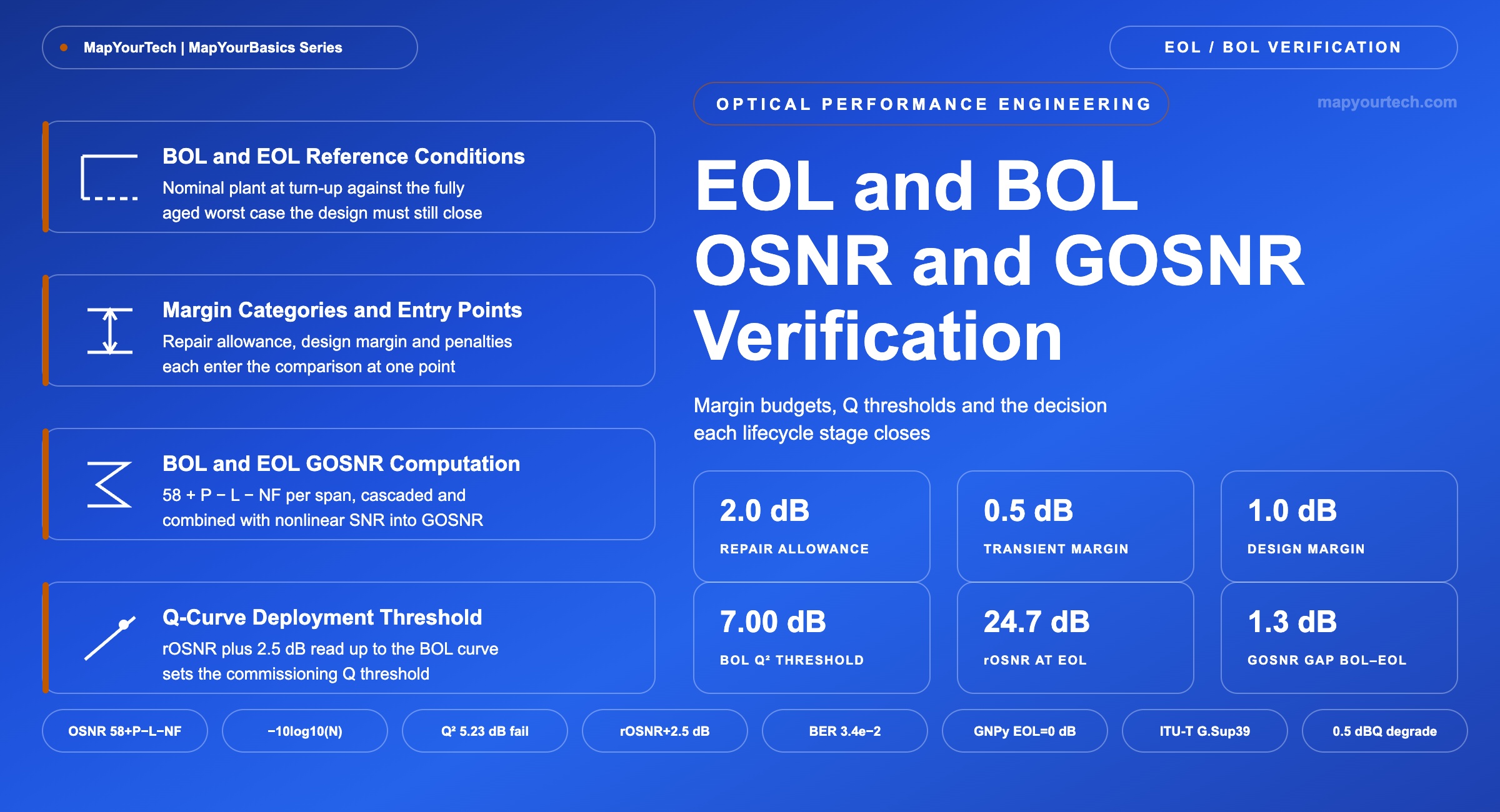
Two evaluations of one route: which allowances load the delivered signal-to-noise ratio, which raise the required value, and how the margin arithmetic closes at both conditions.
The best network design is one that anticipates tomorrow's needs.
What You Will Learn
- Place every margin at its correct entry point: the per-span repair allowance on the delivered side, the design margin on the required side, and impairment penalties as a deduction from path GSNR, with the GNPy parameters that carry each one.
- Compute delivered GOSNR at both life conditions from span loss, launch power, noise figure and nonlinear SNR, and read the EOL margin that decides whether a line rate closes.
- Construct the BOL Q deployment threshold from rOSNR and the 2.5 dB plant allowance on the transponder curve pair, and judge a turn-up measurement against it.
- Select the correct check at each lifecycle stage, design, acceptance and in-service, together with the action each verdict triggers.
- Recognize the two standard double-counting errors: adding transponder ageing on top of the EOL curve, and validating turn-up against the EOL prediction.
1. Introduction
A route is evaluated twice before it is built. Once against the fiber plant as it will be measured on the day of turn-up, and once against the same plant after a service life of cable repairs, connector re-mating, amplifier pump ageing and transceiver drift. Those two evaluations are beginning of life (BOL) and end of life (EOL), and the difference between them is the whole subject of margin allocation.
The two numbers answer different questions. The BOL figure states what the receiver should report at commissioning; the EOL figure states whether the design still closes at the worst plant condition the operator is prepared to underwrite, and it is the one that decides the line rate. Confusing them produces two recognizable errors: a turn-up that appears to have several decibels of unexpected headroom because the measurement was checked against the EOL prediction, and a route that passes acceptance and fails in year eight because only the BOL case was ever run.
This article defines both conditions for optical signal-to-noise ratio (OSNR) and for generalized OSNR (GOSNR), separates the allowances that load the delivered side from those that raise the required side, shows where each one is applied in a planning tool, works a six-span 400 Gb/s budget through both conditions with the arithmetic exposed, and closes with the Q-curve construction that turns an EOL requirement into the Q threshold a commissioning test is run against.
2. Beginning-of-Life and End-of-Life Reference Conditions
Beginning of life is the delivered OSNR or GOSNR computed with the plant at its commissioned condition: measured span losses, the as-built splice and connector count, amplifier noise figures at nominal, and the transceiver at its nominal required OSNR. End of life is the identical route computed with every lifetime allowance applied at once. Neither is a measurement; both are design states of the same model.
Degradation enters on two independent sides of one comparison, and keeping them separate is what makes the arithmetic auditable. On the delivered side, each cable repair inserts a splice pair and a length of slack, so span loss rises monotonically over the life of a buried route; connectors accumulate insertion loss through re-mating and contamination, and a single mating that a microscope check would have caught can cost around 0.9 dB, as the published treatment of connector contamination shows. Amplifier pumps age, raising noise figure. On Raman-amplified spans the effect compounds: pump power is held constant over life, so a higher fiber loss raises the effective noise figure of the Raman stage rather than reducing its gain (vendor claim, from one optical vendor's link-budget documentation).
On the required side the transceiver becomes less tolerant. Manufacturing distribution, temperature range, converter and quantization drift, laser and filter centre-frequency ageing, and polarization-dependent loss events that a short lab test never samples all raise the OSNR the modem needs at the forward-error-correction (FEC) limit. Two of those, the filter penalty and the polarization-dependent loss penalty, are explicitly larger at EOL than at start of life in vendor link-budget models (vendor claim). This is also why a datasheet figure is often already an EOL number: receiver sensitivities in the ITU-T optical interface Recommendations are defined as end-of-life, worst-case values that already include ageing and temperature margins (standard-specified, ITU-T G-series Supplement 39). Adding a separate transceiver ageing allowance on top of such a figure double-counts it.
Start of life (SOL) and beginning of life (BOL) name the same condition and appear interchangeably in vendor documentation and operator request-for-proposal templates. Some templates further distinguish a no-repair BOL case, modelled without any per-span repair allowance, from a BOL case that already carries it; the distinction only matters if the design record states which convention it used.
Takeaway: BOL and EOL are two evaluations of one model, not a measurement and a prediction. Delivered OSNR falls because the line system degrades; required OSNR rises because the transceiver does. A margin figure is meaningful only when the reader knows which of the two conditions produced it.
3. Margin Categories and Their Entry Points
The published low-margin network design literature separates link margin into three categories, and the split maps cleanly onto the BOL and EOL question. System margin covers physical degradation over the service life and is the entire content of the BOL-to-EOL gap. Design margin covers uncertainty in the model and in the input parameters, and it is present at both conditions because the model is no more accurate on day one than in year fifteen. Unallocated margin is whatever remains at BOL after the design was sized for EOL, and it is the quantity that rate-flexible transceivers exist to harvest.
Each category enters at a different point, which is easiest to state against an open reference implementation. In the Telecom Infra Project's GNPy route-planning library, the span-level ageing allowance is the EOL parameter in decibels: it is added to the fiber output connector loss, so both the design pass and the feasibility check run with span loss plus EOL. Design margin is the separate sys_margins parameter, described as added margin on the minimum required transceiver OSNR. Impairment penalties for chromatic dispersion, polarization mode dispersion and polarization-dependent loss form a third path, accumulated and subtracted from the path GSNR before the comparison. Both parameters default to 0 dB (tool-specified), so a route that closes in an untouched configuration file has been evaluated with no lifetime allowance at all.
| Allowance | Side Loaded | Typical Allocation | Evidence Class |
|---|---|---|---|
| Fiber repair and ageing | Delivered | 2 dB per span, added to span loss | Operator design practice |
| Connector re-mating and patch variance | Delivered | Held inside the per-span allowance, or listed separately | Operator design practice |
| EDFA pump ageing | Delivered | Embedded in the vendor EOL noise-figure model | Vendor claim |
| Raman effective noise-figure rise | Delivered | Route-dependent; grows with fiber loss at fixed pump power | Vendor claim |
| Filter and laser frequency ageing penalty | Required | Larger at EOL than at SOL; inside the vendor penalty set | Vendor claim |
| Polarization-dependent loss penalty | Required | Time-varying; sized for rare events, larger at EOL | Vendor claim |
| Transceiver ageing, temperature and factory distribution | Required | Already inside the specified required OSNR | Standard-specified |
| Design margin for model uncertainty | Required | 1-2 dB added to the required OSNR | Tool parameter, default 0 dB |
Takeaway: Every allowance belongs to exactly one side. Loss allowances load the delivered GOSNR and must be applied before the design pass so that amplifier gains are set for the aged plant; transceiver and model allowances raise the acceptance threshold. An allowance applied to the wrong side still moves the margin by the right amount, but it produces the wrong amplifier settings.
4. BOL and EOL GOSNR Computation
The delivered OSNR of an amplified chain is built span by span from a single relation, then combined across spans in the linear domain. The same formula reference applies unchanged at both conditions; only the span-loss input differs.
Per-span OSNR in the 0.1 nm reference bandwidth
OSNRspan = 58 + Pch − Lspan + GRaman − NF
Where:
58 — quantum-limit constant: the product hν·Bref, photon energy times the 12.5 GHz reference bandwidth at 1550 nm, expressed as a power is −58.0 dBm, and the formula carries its magnitude (theoretical constant).
Pch — per-channel launch power into the span, dBm. Typical range −3 to +2 dBm per channel on C-band terrestrial systems.
Lspan — total span loss including fiber attenuation, splices, connectors and the lifetime allowance, dB. Typical range 15 to 30 dB.
GRaman — on/off Raman gain where a Raman stage is fitted, dB, and 0 dB where it is not. Typical range 8 to 15 dB for counter-propagating pumps.
NF — amplifier noise figure, dB. Typical range 4.5 to 6.5 dB for a C-band EDFA.
Cascade combination and the EOL loss step
1 / OSNRlink = Σ ( 1 / OSNRspan,i ) → OSNRlink = OSNRspan − 10·log10(N) for N identical spans
Lspan,EOL = Lspan,BOL + Mrepair
Where:
N — number of amplified spans on the path. The reciprocal sum is the general form; the 10·log10(N) shortcut holds only when the per-span values are equal.
Mrepair — per-span lifetime loss allowance, dB. Commonly 2 dB per span in operator link modelling.
Generalized OSNR and the margin at each condition
1 / GOSNR = 1 / OSNRASE + 1 / SNRNLI
Margin = GOSNR − ( ROSNR + Mdesign + Σpenalties )
Where:
OSNRASE and SNRNLI — the amplified-spontaneous-emission and nonlinear-interference contributions, both in linear units and both referred to the same bandwidth before they are summed. Mixing a 0.1 nm OSNR with a symbol-rate-referenced nonlinear term is the most common arithmetic error in this step.
ROSNR — required OSNR for the selected mode at the FEC limit, dB. For 400 Gb/s dual-polarization 16QAM the published transceiver-class range is roughly 21-23 dB.
Mdesign — design margin for model uncertainty, dB. Typical range 1 to 2 dB.
Formula Sandbox — defaults reproduce Table 2: BOL GOSNR 24.3 dB, EOL GOSNR 23.0 dB, and an EOL margin of 0.5 dB above the 22.5 dB acceptance threshold. The inverse tab solves the same equations backwards for the maximum repair allowance and span count.
Practical Example — six-span 480 km route at 400 Gb/s
Six identical 80 km spans of G.652.D fiber, 0.21 dB/km, with splices and connectors bringing each commissioned span to 18.0 dB. Launch power is 0.0 dBm per channel, amplifier noise figure 5.5 dB, no Raman. The EOL case adds the 2.0 dB per-span allowance and holds launch power constant, because the booster maintains its target output as gain rises. Nonlinear interference is taken as 28.0 dB referred to the same 0.1 nm bandwidth at this launch power (planning-tool value).
| Quantity | BOL (dB) | EOL (dB) | Delta (dB) |
|---|---|---|---|
| Span loss per span | 18.0 | 20.0 | 2.0 |
| Per-span OSNR | 34.5 | 32.5 | -2.0 |
| Cascade term, 10·log10(6) | 7.8 | 7.8 | 0.0 |
| Link OSNR | 26.7 | 24.7 | -2.0 |
| Nonlinear SNR | 28.0 | 28.0 | 0.0 |
| Delivered GOSNR | 24.3 | 23.0 | -1.3 |
| Required OSNR | 21.5 | 21.5 | 0.0 |
| Acceptance threshold | 22.5 | 22.5 | 0.0 |
| Margin above threshold | 1.8 | 0.5 | -1.3 |
Two results deserve attention. The 2.0 dB of added span loss costs exactly 2.0 dB of OSNR, because launch power is held constant and the extra loss is compensated by amplifier gain that also amplifies the noise it now sits above. That one-for-one exchange rate is the single most useful sensitivity in the whole link-engineering dependency framework, and it is independent of span count for identical spans.
The same 2.0 dB costs only 1.3 dB of GOSNR. Nonlinear interference is generated by launch power and fiber effective length, neither of which changed, so its absolute contribution is unchanged while the ASE contribution grew. Combining them as a reciprocal sum then dilutes the OSNR loss. The result is favourable but it depends on an assumption worth stating: the added loss must be lumped, at repair splices and connectors, rather than distributed as a rise in the attenuation coefficient. A distributed rise shortens the effective length and changes the nonlinear term as well, and on Raman-amplified spans it degrades the effective noise figure on top of that, so the GOSNR loss moves back toward the full 2.0 dB.
Takeaway: At constant launch power the OSNR penalty equals the added span loss exactly, one decibel for one decibel. The GOSNR penalty is smaller, 1.3 dB here against 2.0 dB of OSNR, because the nonlinear term does not move with lumped loss. Report both, and state which loss model produced them.
5. Q-Curve Construction of the Deployment Threshold
The transponder side of the same comparison is normally worked on a pair of curves rather than in a table: Q² in decibels against OSNR in the 0.1 nm reference bandwidth, plotted once for a BOL typical transponder and once for an EOL worst-case one. The number a commissioning engineer is handed, a minimum Q at turn-up, is not read off either curve directly. It is constructed from the EOL curve backwards, in three moves, and the same three moves apply at every line rate.
The construction starts at the forward-error-correction limit, because that is the only point on the curve fixed by something other than design policy. Current-generation coherent line interfaces place signal-fail near a pre-FEC bit error rate of 3.4×10⁻², equivalent to Q² = 5.23 dB, and raise the signal-degrade alarm 0.50 dB of Q earlier, at 2.66×10⁻² or Q² = 5.73 dB; an earlier transponder generation used 3×10⁻² and Q² = 5.50 dB (vendor design-rule values, from one optical vendor's deployment-threshold documentation). The OSNR at which the EOL curve reaches that Q is rOSNR, and everything else is built on top of it.
Two quantities are easy to conflate here, and they sit at right angles to each other on the plot. The horizontal separation between the two curves, roughly 2 to 3 dB in published curve pairs, is transponder degradation: ageing, worst-case temperature and factory distribution. The 2.50 dB added at step 2 is fiber-plant degradation: 2.00 dB of fiber repair margin plus 0.50 dB for transients (vendor design-rule values). One is drawn into the curve pair, the other is added to the axis, and counting either one twice removes a decibel of real capacity from the design.
Formula Sandbox — defaults reproduce the 400 Gb/s row of Table 3: BOL OSNR target 27.2 dB and a BOL Q² threshold of 7.00 dB, with 1.08 dB of Q reserved for ageing. The second tab converts a measured turn-up Q back into OSNR headroom on the BOL curve.
| Line-Rate Class | Signal-Fail Q² (dB) | rOSNR at EOL (dB) | OSNR Margin (dB) | BOL OSNR (dB) | BOL Q² (dB) |
|---|---|---|---|---|---|
| 200 Gb/s, earlier generation | 5.50 | 20.40 | 2.50 | 22.90 | 7.50 |
| 400 Gb/s at 56 GBd | 5.23 | 24.70 | 2.50 | 27.20 | 7.00 |
The table shows what stays fixed and what does not. The margin allowance is the same 2.50 dB in both cases, and BOL OSNR is rOSNR plus that allowance in both cases, which is the sense in which the construction is rate-independent. The BOL Q threshold is not the same, and it moves the opposite way from intuition: the 400 Gb/s interface needs 4.30 dB more OSNR yet deploys against a Q threshold 0.50 dB lower. Dividing the Q gained by the OSNR spent gives 0.80 dB per dB for the 200 Gb/s pair and 0.71 dB per dB for the 400 Gb/s pair (derived from the tabulated values), and that flatter slope is the whole explanation. A Q threshold copied from one rate to another is wrong by exactly that difference.
The link back to Figure 1 is direct. Step 2 produces the acceptance threshold on the required side of the margin comparison; step 3 restates it as a Q value, which is what a modem reports and what an acceptance test can be written against. A route that closes on GOSNR but is commissioned against the wrong Q threshold has passed the design and failed the handover.
Takeaway: Build the deployment threshold from the FEC limit outward: rOSNR on the EOL curve, plus the plant margin, then up to the BOL curve. The 2.50 dB allowance transfers between rates unchanged; the resulting Q threshold does not, because the curve slope near the FEC limit differs with baud and modulation.
6. Practical Guidelines for Margin Verification
A design record that carries only one margin figure cannot be audited later. Carry both, with the allowance set that produced each one, and the acceptance test writes itself.
The three checks separate cleanly by lifecycle phase, and each compares a different number against a different threshold: the design pass closes on the EOL GOSNR margin, acceptance closes on the BOL Q threshold, and operation tracks the remaining margin toward the EOL requirement. Figure 4 places the three in sequence, with the inputs each one needs, the procedure it runs, and the action each verdict triggers; the first two lanes are the ones the two Formula Sandboxes above compute.
- Check turn-up against the BOL prediction. The receiver at commissioning sees the commissioned plant. A measured GSNR that exceeds the EOL figure by 3 dB is not surplus capacity; it is the lifetime allowance, already spoken for.
- Read the modem, not the spectrum analyzer. Wavelength-selective-switch filtering carves out the inter-channel noise floor an optical spectrum analyzer interpolates across, so an in-line OSNR reading in a ROADM network is unreliable. The modem-reported GSNR, effective SNR or Q is the number the acceptance threshold was written against.
- Trend the margin, and act on the slope. A margin that drifts downward over months while still positive points to a developing physical fault, most often a degrading connector or a failing pump. That slope is the actionable signal, not the crossing.
- Re-baseline after every repair. Each repair consumes part of the allowance. Recording measured span loss against the design assumption converts an abstract lifetime allowance into a countable remaining budget.
- Harvest unallocated margin deliberately. Rate-flexible transceivers can convert BOL surplus into capacity, and the required-OSNR ladder gives the price of each step. Do it against the BOL number with a written plan for stepping the rate down later, not by quietly reclassifying the EOL allowance as headroom.
- Test the worst span before reaching for a regenerator. If a single span fails on its own at EOL, regeneration placement will not recover the route; the answer is a lower line rate, a physical repair, or a different path.
Two model choices deserve a line in the record. Applying the per-span allowance before the design pass, rather than after, decides whether amplifier gains and launch powers were optimized for the aged plant, and before is the conservative and standard order. On C+L systems, band loading changes over life as well as loss: inter-band Raman transfer makes delivered tilt a function of how much spectrum is lit, so partial-fill and full-fill EOL cases are different design cases and both should be evaluated.
Takeaway: BOL is the acceptance reference, EOL is the design reference, and the gap between them is a budget to be spent knowingly. Trending the measured margin against the BOL prediction is what turns that budget from an assumption into a tracked quantity.
7. Summary
BOL and EOL are two evaluations of one model under different plant assumptions. Delivered OSNR and GOSNR fall over life because span loss rises and amplifier noise figures degrade; required OSNR rises because the transceiver ages, though a datasheet figure specified to the ITU-T convention already contains that allowance. Loss allowances load the delivered side and belong in the design pass; design margin and impairment penalties load the required side.
Reference values from the example above: a 2.0 dB per-span lifetime allowance, one decibel of OSNR lost per decibel of span loss at constant launch power, 1.3 dB of GOSNR lost against 2.0 dB of OSNR when the added loss is lumped, and a 1.0 dB design margin sitting on the required side at both conditions. For the next step, the optical link OSNR simulator runs the cascade arithmetic across unequal spans, and the treatment of Q-factor covers the conversion between a decibel margin and a pre-FEC bit error rate.
8. References
- ITU-T G-series Supplement 39 — Optical System Design and Engineering Considerations, ITU-T Study Group 15.
- Telecom Infra Project OOPT/PSE Working Group — GNPy: Optical Route Planning and Performance Estimation Library, Project Documentation.
- Y. Pointurier — Design of Low-Margin Optical Networks, Journal of Optical Communications and Networking.
- Sanjay Yadav, "Optical Network Communications: An Engineer's Perspective" — Bridge the Gap Between Theory and Practice in Optical Networking.
Related Articles on MapYourTech