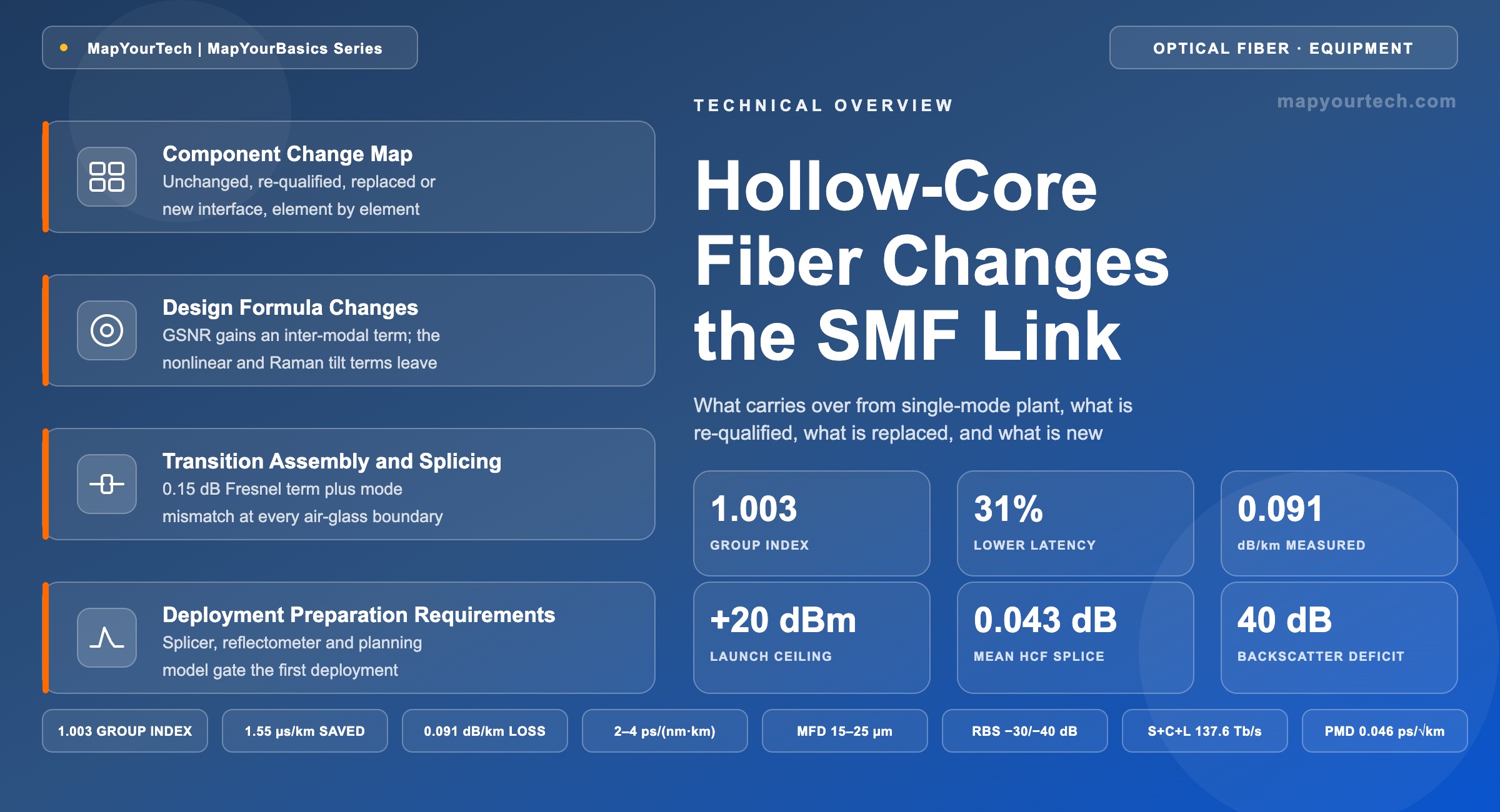
Hollow-Core-Fiber-Driven Changes to the Current SMF Link
Which components carry over unchanged from single-mode plant, which are re-qualified at a new operating point, which are replaced outright, and which impairments enter the budget for the first time.
Measure the path you will deploy, not the one you modelled.
1. Introduction
A hollow-core span replaces one element of an optical link and leaves most of the equipment list alone. The transponder, the multiplexer, the wavelength selective switch (WSS), the passive couplers and the erbium-doped fiber amplifier all terminate on single-mode pigtails, and none of them touches the air core. What does change sits in three places: the two interfaces on either side of the span, the operating points the line system is configured to, and the instruments used to prove the plant is good.
Deployment volume has moved past the pilot stage. Microsoft reports more than 1,280 km of hollow-core fiber (HCF) carrying live Azure traffic with a 15,000 km build announced for late 2026, and Amazon Web Services has disclosed links at roughly ten data centers for availability-zone interconnect (both vendor-published). euNetworks has carried financial-trading traffic on hollow-core routes since April 2021, about 87 km across London and continental segments (vendor-published). Prysmian and Relativity Networks have built a 10 mm cable holding 24 hollow-core fibers and jetted it at up to 107 m/min (vendor claim). The technology still sits well under 0.1% of installed fiber, so almost every deployment is an insertion into plant designed around standard single-mode fiber (SMF) parameters.
This overview walks the link element by element and states, for each one, whether the hardware carries over, whether it carries over at a different operating point, or whether it is replaced. Background on the guidance mechanism itself is covered in the MapYourTech treatments of hollow-core fiber fundamentals and deployment readiness.
Takeaway: Four component classes describe the whole link. Unchanged hardware on single-mode ports, unchanged hardware at a new operating point, replaced hardware at the air-glass boundary, and two impairments that have no equivalent in solid-core plant.
2. Group Index and Air-Core Guidance Definitions
An anti-resonant hollow-core fiber guides light in an air-filled core ringed by thin glass capillaries that reflect by anti-resonance rather than by total internal reflection. Its group index, the ratio of the vacuum speed of light to the group velocity of the guided mode, measures about 1.003 against 1.468 for a silica core. That single number sets propagation delay, and it is the origin of the latency result.
The capillary walls behave as Fabry-Perot reflectors. Resonance wavelengths follow λm = 2t√(n² − 1)/m, with t the wall thickness, n the refractive index of silica near 1.45, and m the resonance order. Wall thickness of 480–550 nm places the first-order resonance below 1550 nm and opens a low-loss window spanning the C- and L-bands (standard-specified geometry reported in the anti-resonant fiber literature). Confinement loss scales as (λ/Rcore)4, so a larger core lowers loss and at the same time admits more higher-order modes. That trade-off drives most of the fiber design work.
2.1 Commonly Confused Adjacent Quantities
Group index against refractive index. The refractive index of air is 1.0003 at 1550 nm, but the guided mode is not pure air: a small fraction of the field overlaps the glass membranes and the waveguide itself contributes dispersion, so the measured group index of cabled hollow-core fiber lands near 1.003 rather than 1.0003 (measured; two cabled samples reported 1.003 and 1.005). Propagation delay follows the group index, not the material index.
Core diameter against mode field diameter. The mode field diameter is about 70% of the core diameter in current anti-resonant designs, so a 30 µm core carries a 21 µm mode (measured). Reported telecom fibers run 15–25 µm mode field diameter against 10.4 µm for SMF-28 at 1550 nm. Every interface loss figure derives from that ratio, not from the core size.
Attenuation against backscatter coefficient. These are independent properties. Hollow-core fiber can carry less loss per kilometer than silica while returning 30–40 dB less Rayleigh backscatter (measured), because the scattering that an optical time domain reflectometer (OTDR) relies on comes from air molecules and capillary-wall roughness rather than from frozen density fluctuations in glass. A fiber can be excellent to transmit through and nearly invisible to a reflectometer at the same time.
t / L = ng / c = 3.3356 × ng µs/km
- t — one-way propagation delay, µs
- L — route length, km
- ng — group index, dimensionless; 1.003 hollow-core, 1.468 G.652.D single-mode
- c — vacuum speed of light, 299,792,458 m/s, giving 3.3356 µs/km per unit of group index
Practical Example — latency on a 40 km metro route
Single-mode fiber at a group index of 1.468 gives 1.468 × 3.3356 = 4.90 µs/km, so 40 km costs 195.9 µs one way. Hollow-core fiber at 1.003 gives 3.35 µs/km, so the same route costs 133.8 µs. The saving is 1.55 µs/km, 62.1 µs one way and about 124 µs on the round trip. Field measurements of cabled hollow-core fiber report 1.54 µs/km and a 31% reduction, which agrees with the arithmetic to within the group-index measurement spread (measured).
Takeaway: Group index sets delay, mode field diameter sets interface loss, and backscatter coefficient sets what a reflectometer can see. The three are separate quantities, and each one drives a different part of the hardware decision.
3. Component Change Map Across the Link
Only components that physically contact the air core need new hardware. Everything upstream and downstream of the two transition assemblies presents a single-mode interface and carries over from existing plant, though several elements operate at settings that a solid-core design would not use.
3.1 Transmit and Receive Terminals
Coherent transponders and pluggables carry over as they are. The optics, the modulator, the receiver front end and the digital signal processing (DSP) engine all present a single-mode interface, and no part of the module is aware of what medium follows it. Three settings change. Chromatic dispersion accumulation drops from about 17 ps/(nm·km) on G.652.D to 2–4 ps/(nm·km) (measured), narrowing the receiver compensation window by roughly a factor of five and cutting the direct-detection equalizer tap count by 3–6× (analytical result from published modeling). Launch power rises, because the air core carries a nonlinear coefficient roughly three orders of magnitude below silica, admitting per-channel powers of +10 to +20 dBm without meaningful nonlinear degradation (analytical bound supported by published transmission results). And the transmitter takes on a task it does not have on silica: shaping the spectrum around residual gas absorption lines.
That last point produces the largest terminal-side change. Residual carbon dioxide, carbon monoxide and water vapor trapped in the core produce narrow absorption lines a few GHz wide, deepest in the L-band, measured at up to about 0.08 dB/km at the peak (measured). An optical amplifier cannot flatten a line that narrow, so every mitigation sits at the transmitter or in digital signal processing. Pre-emphasis against the known loss spectrum extended reach from 150 km to 300 km in one 89.6 GBd probabilistically shaped 64-state quadrature amplitude modulation (64QAM) experiment, digital subcarrier multiplexing places subcarriers clear of the peaks, and per-channel launch-power control held more than 1.5 dB of Q-factor margin on every channel of a fully loaded 32 × 800G C-band system over a 442.7 km three-span hollow-core link (measured).
3.2 Multiplexers, ROADMs and Passive Components
Multiplexers, demultiplexers, wavelength selective switches, arrayed waveguide gratings (AWG), splitters, couplers, optical channel monitors and optical supervisory channel filters all carry over without modification. Every port on a reconfigurable optical add-drop multiplexer (ROADM) is single-mode, and the hollow-core fiber begins after the line port. The qualification is location rather than technology. No hollow-core equivalent of these devices exists: there is no fused coupler, no planar splitter and no fiber Bragg grating that can be formed in an air core. Any of them placed in line on a hollow-core span therefore needs a transition on each side, at roughly 0.44 dB per interface (analytical) plus two further mode-coupling sites that feed inter-modal interference. Mid-span taps and in-line couplers are designed out rather than reused, which is part of why monitoring moves to a witness fiber or an end-of-link element. The add-path power budget in a high-degree ROADM is affected only indirectly, through the higher launch power the span will accept.
Two node-level settings change even though no hardware does. The wavelength plan avoids or de-rates L-band slots that sit on gas absorption lines, and every planned wavelength is checked against the anti-resonant window of the specific fiber, which is not a constant across products: one commercial hollow-core cable specifies an operating window greater than 10 nm centered on 1550 nm, while a broadband double-nested design measures below 0.1 dB/km from 1481 to 1625 nm and below 0.2 dB/km across 66 THz (vendor-published and measured). That check includes the optical supervisory channel, which conventionally runs at 1510 nm or 1625 nm and falls outside a narrow window. Some anti-resonant designs also carry resonant loss peaks inside their nominal window, so the acceptance document specifies a spectrum rather than a single attenuation figure.
One node-level design option opens up. Backscatter 30–40 dB below single-mode levels reduces the coherent crosstalk that normally limits sending both directions on one fiber, which makes bidirectional operation practical on a single strand. Reported results include S+C+L bidirectional transmission beyond 550 Tb/s over 109 km of anti-resonant hollow-core fiber (measured) and a bidirectional passive optical network over 22 km of anti-resonant hollow-core fiber at 200 Gb/s downstream and 50 Gb/s upstream, exceeding the ITU-T N2 class power budget (measured). Halving strand count on a subsea or duct-constrained route changes cable economics, and it requires circulators and directional filters at the node rather than any new component technology. Those elements are not free: published system modeling budgets 0.7 dB per circulator and 1.0 dB per band multiplexer, and a reported 121.6 km loop measured about 1 dB per circulator (measured and simulated).
3.3 Optical Amplification
Erbium-doped fiber amplifiers carry over unchanged as devices. The gain block is a length of doped fiber between single-mode pigtails, and it neither knows nor cares about the transmission medium. Two design consequences follow all the same.
Distributed Raman amplification is not available in the span. Raman gain requires the pump and the signal to overlap in silica, and an anti-resonant hollow-core fiber places over 99% of the field in air, which removes the gain medium. The same absence removes inter-channel stimulated Raman scattering (SRS), so SRS-induced tilt, pre-tilt and the dynamic gain equalization a wide C+L design normally carries drop out of the plan. Lower span loss and higher launch power replace the missing distributed gain. Real-time unrepeatered transmission has reached 726.1 km at 400G, 611.9 km at 800G and 436.1 km at 1.2T using high-power erbium amplifiers only, with no Raman pumps and no remote gain units (measured). Single-mode demonstrations in the same 600 km class need high-power boosters plus remote optically pumped amplifiers (ROPA) fed over dedicated fibers (vendor-published), so the hollow-core version removes both the mid-span engineering and the pump-feed fiber.
Amplifier selection shifts toward higher output power classes. With span loss roughly halved and nonlinear penalty removed, the booster becomes the limiting element rather than the fiber, and demonstrations have run optimum launch powers up to 34.77 dBm for a 1.2T channel (measured). That level requires different connector cleanliness, optical return loss and laser safety practice than a +18 dBm C-band booster does. The gain plan needs checking at the other end of the range as well: halved span loss means the in-line amplifier runs at lower gain, and an erbium amplifier operated near or below about 10 dB of gain gives back in noise figure part of what the shorter span budget bought (published link modeling).
3.4 Fiber Plant, Splices and Terminations
Duct practice carries over; the cable itself is a new product. Current telecom-oriented anti-resonant fibers hold the 125 µm glass and 250 µm coating geometry of G.652 fiber, so loose-tube constructions, 900 µm buffers, microduct sizing, jetting equipment and enclosure hardware stay as they are. What is new sits inside the sheath: hermetic termination at both ends to keep gas and water out, water-blocking construction that has to hold against capillary ingress rather than only against longitudinal water travel, and a cabling process that can raise attenuation and reveal polarization-mode dispersion which spooling had masked. Minimum bend radius of 15–30 mm is tighter than single-mode practice and is usually the binding mechanical limit in brownfield routes rather than cable diameter (measured design values).
Splicing is where hardware changes outright. A standard telecom fusion splicer collapses the capillary structure, so hollow-core work uses machines with rotational alignment to about 0.1° and controlled arc or pressurized heating that keeps the tubes open. Reported hollow-core to hollow-core results include a 0.043 dB mean over 30 trials with 100% success on a field-capable splicer (measured), against a deployed mean of 0.16 dB on production routes (vendor-published). Practice around the splice changes as well: figure-eight coiling to remove torsional stress, epoxy-sealed end caps, splicing at 40% relative humidity or below, and IP68 closures.
The hollow-core to single-mode transition is the one interface with no equivalent in existing plant, and it carries two loss terms. The Fresnel term is fixed by the index step between air and silica at about 0.15 dB per interface, removable only by an anti-reflection coating or an angled face (standard-specified). The mode-mismatch term follows the overlap integral of the two fields, and the design result is counterintuitive: coupling loss is lowest when the single-mode side has a mode field diameter about 83% of the hollow-core value rather than an equal one, because that reduces overlap with the core wall region. Thermally expanded core fiber, graded-index segments and tapers all serve as mode-field adapters, and interconnection now reaches below 0.2 dB insertion loss with back-reflection below −60 dB (measured). Commodity LC and MPO connectors are not yet in production quantities, so panels use factory-prefabricated adapters, covered in the MapYourTech treatments of splicing and connectorization and patch panel and adapter design.
A breached hollow core draws water in by capillary action, and a flooded section is opaque at telecom wavelengths. Trapped water cannot be driven out by splicing, so a flooded segment is replaced and re-terminated rather than repaired in place. On flood-prone outside-plant routes this changes the restoration plan, not only the repair kit.
3.5 Test, Monitoring and Fault Location
Reflectometry is the instrument class that changes most. Backscatter in hollow-core fiber comes from two sources: moving air molecules, which sit about 27 dB below the Rayleigh level of solid-core fiber, and static capillary-wall roughness, a further 15 dB below that (measured). The combined backscatter coefficient runs 30–40 dB under single-mode fiber, and the displayed OTDR trace sits 14–20 dB lower, which compresses usable dynamic range. The coefficient also varies along the fiber with microstructure and gas conditions, so trace slope can change without any change in link loss.
Three practical consequences follow. Single-ended trace-shape analysis is not reliable on hollow-core spans, so bidirectional acquisition combined as (A→B − B→A)/2 is used to cancel backscatter asymmetry and separate real loss from backscatter drift. Continuous in-service monitoring moves to a stable end-of-link reference element whose return level tracks total insertion loss at about 1 dB absolute accuracy, against better than 0.3 dB from a full bidirectional measurement, and that choice also avoids the in-band multiplexer an in-line tap would require. And hollow-core instruments have reached the market: a bidirectional OTDR kit with roughly 150 km range and 46 dB dynamic range launched in September 2025, an all-in-one test and certification package followed in January 2026, and optical frequency domain reflectometry now covers distributed characterization at sub-millimeter resolution over 5 km and 3 m resolution over 100 km (vendor-published and measured). Monitoring architecture is treated separately in the MapYourTech article on in-service monitoring design.
Optical spectrum analyzers (OSA), optical channel monitors (OCM) and power meters carry over for per-channel power, because they measure at single-mode ports, and per-channel equalization loops keep working with the target profile recomputed for the new span loss and any gas-line offsets. Resolution is the exception. A gas absorption line is about 1 GHz wide, near 8 pm at 1550 nm, which sits under the 20–50 pm resolution of a grating spectrum analyzer and well under the resolution of any ROADM channel monitor. Characterizing those lines takes a swept tunable laser system at about 1 pm resolution, and the inter-modal interference sweep method uses 0.2 pm steps over a 2 nm window (measured line width and sweep method; instrument resolutions vendor-specified).
| Component | Change class | What changes |
|---|---|---|
| Coherent transponder | Re-qualified | Dispersion compensation window, launch power target, spectral pre-emphasis or subcarrier placement around gas lines, and margin held for impairments the DSP cannot equalize |
| Direct-detection optics | Re-qualified | Equalizer tap count falls 3–6× and dispersion-limited reach extends 4–8×; accumulated multipath interference must stay below −30 dB |
| Mux, demux, AWG, filters | Unchanged | Nothing; every port is single-mode and every device sits at a node |
| ROADM and WSS | Unchanged in hardware | Wavelength plan avoids gas-affected slots and is checked against the fiber's anti-resonant window; bidirectional single-strand operation becomes a design option |
| Couplers, splitters, taps | Unchanged at the node, re-sited on the span | Device technology unchanged, but no hollow-core equivalent exists; an in-line tap costs a transition pair, so mid-span taps are designed out |
| Optical supervisory channel | Re-sited or retuned | 1510 nm and 1625 nm can fall outside a narrow anti-resonant window; the OSC moves in-band, onto a companion single-mode fiber, or to a wavelength inside the window |
| Erbium amplifier | Re-qualified | Higher output power class at one end; at the other, halved span loss pushes in-line gain toward the range where noise figure degrades |
| Raman amplifier | Removed | No silica overlap in the span, so distributed Raman gain is unavailable and SRS tilt correction drops out; a hybrid span with single-mode fiber at the tail is the workaround |
| Duct, jetting, enclosures | Unchanged | Nothing; 125/250 µm geometry preserves microduct sizing and installation equipment |
| Cable | New product | Hermetic termination, water blocking against capillary ingress, and a cabling process that can raise loss and unmask PMD; bend radius limit 15–30 mm |
| Fusion splicer | Replaced | Rotational alignment and controlled heating; an unmodified splicer collapses the capillaries |
| Splice closure and end cap | Replaced | Hermetic epoxy end caps as a lifetime seal, humidity-controlled splicing, IP68 closures |
| Connector and adapter | New interface | Mode-field adapter plus angled or coated face; no commodity LC or MPO part yet |
| Optical distribution frame | Replaced | Factory-built transition assemblies, sealed terminations, dedicated test port |
| OTDR | Replaced | Hollow-core bidirectional instrument; single-ended trace-shape analysis is not reliable |
| OSA, OCM, power meter | Unchanged for power, insufficient for spectrum | Per-channel power measurement is unaffected; gas lines near 8 pm wide sit below grating-analyzer resolution and need a swept tunable laser system |
Takeaway: The active line system carries over. What is replaced is everything within a meter of the air-glass boundary, plus the reflectometer, and what is re-qualified is every power, gain and dispersion setting that assumed silica.
4. Performance Advantages and Design Limits
Four parameters improve by large factors and two new impairments appear. Attenuation, group index, chromatic dispersion and nonlinear coefficient all move in the design engineer's favor; gas-line absorption and multipath interference (MPI) move against it, and neither has an equivalent in solid-core plant.
| Parameter | Anti-resonant hollow-core | G.652.D single-mode | Design consequence |
|---|---|---|---|
| Attenuation | 0.09–0.15 dB/km in production; 0.04–0.05 dB/km best reported (measured) | 0.19–0.21 dB/km cabled (measured) | Span loss roughly halved; amplifier sites removed |
| Group index | 1.003 (measured) | 1.468 (measured) | 1.55 µs/km less delay, a 31% reduction |
| Chromatic dispersion | 2–4 ps/(nm·km) (measured) | About 17 ps/(nm·km) (standard-specified) | Smaller compensation window; fewer equalizer taps |
| Nonlinear coefficient | About three orders of magnitude below silica (theoretical limit) | Reference | +10 to +20 dBm per channel usable |
| Polarization mode dispersion (PMD) coefficient, cabled | 0.046 ps/√km (measured) | 0.1 ps/√km link design value (standard-specified) | Headroom at high baud rate, and for direct detection |
| Mode field diameter | 15–25 µm (measured) | 10.4 µm (standard-specified) | Mode-field adapter at every transition |
| Rayleigh backscatter | 30–40 dB below single-mode fiber (measured) | Reference | New reflectometry; bidirectional single-strand operation |
| Thermal coefficient of delay | About 20× lower (measured) | Reference | Less clock phase tracking in switched fabrics |
| Low-loss window | Below 0.1 dB/km across 18 THz; below 0.2 dB/km across 66 THz (measured) | C+L covers about 11 THz | Roughly 50% more spectrum than super-C plus super-L combined |
| Minimum bend radius | 15–30 mm for acceptable loss (measured) | Macrobend specified at 30 mm; G.657 classes to 7.5–15 mm (standard-specified) | Routing constraint in panels and closures |
| Gas-line absorption | Narrow peaks to about 0.08 dB/km, deepest in the L-band (measured) | None | New budget entry; purge or compensate digitally |
| Multipath interference | −52 to −73 dB/km reported across designs (measured) | None | New budget entry; sets modal purity requirement |
| Installed fiber cost | About $5–10 per meter (published market analysis) | About $0.10 per meter (published market analysis) | A 50–100× premium, offset only where latency or reach pays |
4.1 Multipath Interference as a New Budget Entry
Low-loss hollow-core fibers are not strictly single-moded. A core small enough to guide one mode alone would carry high confinement loss, so telecom designs use a larger core and suppress higher-order modes by differential modal attenuation instead. Reported values include differential modal attenuation above 6,500 dB/km for the LP11 mode, and differential attenuation above 12 dB/km is enough to hold interference-induced crosstalk below the −30 dB multipath interference threshold that four-level pulse amplitude modulation (PAM4) requires (measured and analytical). The exposure is that modal purity depends on geometry being preserved end to end: mechanical stress, tight bends or temperature cycling deform the capillary structure locally and raise multipath interference, and long-term reliability data under the standard cable test protocols is still accumulating.
Practical Example — 80 km span budget on hollow-core against single-mode fiber
Take an 80 km duct route. On cabled G.652.D at 0.21 dB/km, fiber loss is 16.8 dB, and with two connector pairs and field splices at about 1.0 dB the span presents roughly 17.8 dB. On production hollow-core fiber at 0.12 dB/km, fiber loss is 9.6 dB; add two hollow-core to single-mode transitions at 0.25 dB each and eight field splices at 0.1 dB, and the span presents about 10.9 dB. The span budget improves by 6.9 dB. Launch power adds to that: a practical +3 dBm per channel on silica against +10 dBm on hollow-core contributes a further 7 dB, for roughly 14 dB of additional system margin. That figure is what removes an in-line amplifier site on a two-span route, or extends an unrepeatered reach, rather than any change in the amplifier or transponder itself. Verify each term against the plant before use, following the fiber characterization thresholds in the DWDM commissioning checklist.
Takeaway: The gain is roughly 7 dB of span loss and roughly 7 dB of launch power headroom, spent either on removing amplifier sites or on reach. The cost is a 50–100× fiber price and two impairments that need explicit budget lines.
5. Design Formula Changes for Hollow-Core Spans
Most link-design formulas keep their form on a hollow-core span and change only their inputs. Three change form, because a noise term appears or disappears, and one has no single-mode equivalent at all. A planning tool loaded with a hollow-core attenuation figure and nothing else will return an optimistic answer, because it drops the two terms that only exist on this medium.
5.1 Noise Terms Entering and Leaving the Budget
The generalized signal-to-noise ratio (GSNR) is the planning metric that carries every noise contribution along a path, and its span-level definition gains a third term on hollow-core fiber. Published network-planning models for mixed routes now write the span quality of transmission with an inter-modal interference (IMI) power alongside amplified spontaneous emission (ASE) and nonlinear interference (NLI), and the path composition rule remains the reciprocal sum it has always been.
GSNRspan = Psignal / (PASE + PNLI + PIMI)
1/GSNRpath = Σspans 1/GSNRspan + Σnodes 1/OSNRnode
- PASE — amplifier noise power in the reference bandwidth, W; unchanged in form, lower in value because span loss falls
- PNLI — Gaussian-noise nonlinear interference, W; falls to a negligible contribution on hollow-core fiber
- PIMI — inter-modal interference power, W; zero on single-mode fiber, non-zero on every hollow-core span and rising linearly with length
- OSNRnode — optical signal-to-noise ratio (OSNR) contributions at the add, drop and intermediate ROADMs, unchanged
- Residual margin follows as RM = GSNRpath − ROSNRB2B − Msys, in dB, with ROSNRB2B the required OSNR at the receiver in back-to-back operation and Msys the system margin
The nonlinear term does not vanish by assumption; it falls because the nonlinear coefficient does. With γ = 2πn2/(λAeff), the air core changes both factors: a nonlinear index near 2.2 × 10⁻²³ m²/W against 2.2 × 10⁻²⁰ m²/W for silica, and an effective area of roughly 300–800 µm² against 80 µm² (measured and standard-specified). Published hollow-core transmission simulations therefore use γ values three to four orders of magnitude below the roughly 1.3 /(W·km) of G.652.D. One detail runs the other way. Gaussian-noise efficiency scales approximately as γ²/|β2|, so the low dispersion of hollow-core fiber raises efficiency for a given γ. The reduction in γ² covers that by a wide margin, but a tool configured with the correct dispersion and a default silica γ will report nonlinear penalties that are wrong by orders of magnitude.
Inter-modal interference replaces nonlinearity as the impairment that scales with launch power and length. It arises where a fraction of the fundamental mode couples into a higher-order mode at a splice, a connector or a structural perturbation, then produces a beat term against the fundamental mode at the receiver. Reported coupling per interface is near −35 dB for an optimized hollow-core to single-mode splice and −20 to −25 dB for an unoptimized one (measured), which is why interface quality and fiber uniformity are the same problem. No standardized measurement method exists yet; the sweep-frequency method is the one in common use, and the resulting figure is quoted per kilometer so it can be accumulated along a link.
IMI (dB/km) = 10·log10[(σ/Pavg)² / (2L)]
MPIlink (dB) = IMI (dB/km) + 10·log10(L)
- σ — standard deviation of received power across a swept window, typically 2 nm at 0.2 pm steps
- Pavg — mean received power across the same window
- L — fiber length, km
- Reported fiber values run −52 to −73 dB/km across designs; a 266 km spliced link measured −68.8 dB/km (measured)
- PAM4 direct detection requires the accumulated figure to stay below −30 dB (analytical)
Practical Example — inter-modal interference accumulation on a 300 km link
Take spans of anti-resonant fiber measured at −65 dB/km. Over 300 km the accumulated figure is −65 + 10·log10(300) = −65 + 24.8 = −40.2 dB, which leaves about 10 dB of headroom against the −30 dB threshold. The exposure is not the average but the worst span. In a reported splicing study, three fiber groups at roughly −65 dB/km held −65.9 dB/km when spliced together, and adding a single group measured at −53.9 dB/km pulled the whole link above −60 dB/km (measured). One poor span sets the link figure, so every span is screened rather than sampled.
5.2 Launch Power Ceiling and Its Limiting Mechanism
The mechanism that caps per-channel launch power changes identity. On G.652.D the ceiling is Kerr nonlinearity, and practical operation sits near +3 dBm per channel (analytical bound supported by deployed practice). On hollow-core fiber the Kerr term leaves the budget and stimulated Brillouin scattering stops binding, because the pump has almost no silica to interact with. What remains is inter-modal interference, together with the ratings of connectors, splices and amplifiers, so the ceiling lands between +10 and +20 dBm in general design and higher in specific experiments.
Two consequences follow for the arithmetic. Every decibel of extra launch power converts directly into span budget rather than into nonlinear interference, which is why the amplifier and not the fiber becomes the limiting element. The same margin can be spent on modulation order instead of reach: beyond 1 Tb/s per wavelength with probabilistically shaped 144-state QAM has been demonstrated over 100 km of anti-resonant fiber with no measurable nonlinear penalty (measured). And the optimum launch power is no longer found by balancing amplified spontaneous emission against nonlinear interference; it is found by increasing power until either the inter-modal ceiling or a component rating is reached. The MapYourTech treatment of the GSNR budget for mixed hollow-core and single-mode routes works that composition through span by span.
5.3 Span Power Budget with the Transition and Gas Terms
The span power budget keeps its additive form and takes two new entries. The first is the pair of hollow-core to single-mode transitions, one at each end, which has no counterpart on an all-silica span. The second is gas-line absorption, which is wavelength-dependent and therefore turns a single attenuation coefficient into a spectrum.
Lspan(λ) = [αfiber + αgas(λ)]·L + ns·αsplice + nc·αconn + 2·αtrans
αtrans = αFresnel + αmismatch, αFresnel = −10·log10[1 − ((n1 − n2)/(n1 + n2))²]
- αfiber — 0.09–0.15 dB/km in production, against 0.19–0.21 dB/km cabled G.652.D
- αgas(λ) — narrow absorption lines near 1 GHz wide at roughly 40 GHz spacing, to about 0.08 dB/km at the peak, concentrated in the L-band
- αFresnel — 0.15 dB per interface for n1 = 1.45 and n2 = 1.0, removable only by an anti-reflection coating or an angled face
- αmismatch — from the transverse overlap integral of the two fundamental modes; minimized at a single-mode mode field diameter near 83% of the hollow-core value
- ns, nc — splice and connector counts; roughly one splice per 2 km of deployed hollow-core cable (published cost model)
Practical Example — choosing the single-mode side of a transition
For a hollow-core fiber with an 18 µm mode field diameter at 1550 nm, matching the single-mode side at 18 µm gives about 0.50 dB of mode-mismatch loss. Setting the single-mode mode field diameter to roughly 15 µm, near 83% of the hollow-core value, lowers mismatch to about 0.29 dB, because the smaller field overlaps less with the core wall region where the hollow-core mode is strongly position-dependent (analytical, published coupling analysis). Adding the 0.15 dB Fresnel term gives 0.44 dB against 0.65 dB, so the deliberate mismatch saves 0.42 dB across the two transitions of a span. Matching the two fibers by intuition costs more than accepting the asymmetry.
Gas absorption enters the budget differently from every other loss term, because it is narrow enough to sit inside a single channel rather than across the band. It is modelled as a product of Lorentzian notches in the frequency domain, and the OSNR penalties from individual lines add linearly once each line is mapped to a penalty by its depth. That linearity is what makes a single field measurement useful: a one-shot characterization on one length of a given fiber type can be re-scaled to predict the penalty on other lengths of the same type before a wavelength plan is committed (measured).
5.4 Formula Inventory and Change Class
| Quantity and form | Change class | What moves |
|---|---|---|
| Propagation delay, t = ngL/c | Input only | Group index 1.468 → 1.003; 4.90 → 3.35 µs/km |
| Span loss, αL + splices + connectors | New terms | Adds two transition losses and a wavelength-dependent gas term |
| Transition loss, αFresnel + αmismatch | No single-mode equivalent | 0.15 dB fixed plus overlap integral; optimum mode field diameter ratio 0.83 |
| OSNR after N spans, P − Lspan − NF + 58 − 10log10N | Input only | Span loss roughly halved, launch power 7–17 dB higher |
| Span GSNR, P/(PASE + PNLI) | New term | Adds PIMI, non-zero only on hollow-core spans |
| Nonlinear coefficient, γ = 2πn2/(λAeff) | Input only | Falls three to four orders of magnitude below 1.3 /(W·km) |
| Brillouin threshold, Pth ≈ 21Aeff/(gBLeff) | Term leaves | No longer sets the launch ceiling; the pump has no silica interaction |
| Inter-channel Raman tilt | Term leaves | Falls to zero, and with it pre-tilt and dynamic gain equalization |
| Dispersion accumulation, D·L, and DSP tap count | Input only | D 17 → 2–4 ps/(nm·km); equalizer taps fall 3–6× |
| Direct-detection fading null, f = √(c/2DLλ²) | Input only | First null moves from about 10 GHz to 20–28 GHz at 40 km |
| PMD accumulation, DGD = PMDcoef√L | Input only | Cabled coefficient 0.1 → 0.046 ps/√km |
| Thermal delay drift, Δτ = (dτ/dT)·L·ΔT | Input only | About 40 → 2 ps/(km·°C) bare, near 6 ps/(km·°C) coated |
| Differential delay on a mixed path | New quantity | (ng,SMF − ng,HCF)L/c = 1.55 µs/km between media |
| Backscatter and bidirectional crosstalk | Input only | Coefficient near −100 dB/m, about 30 dB below single-mode fiber |
Takeaway: Two terms leave the budget and two arrive. Nonlinear interference and Raman tilt go; inter-modal interference and a wavelength-dependent gas loss arrive, and the transition pair is a loss item with no single-mode counterpart at all.
6. Deployment Scenarios and Typical Configurations
Financial trading was the first paying application and remains the clearest. euNetworks placed the first commercial route between a London data center and the London Stock Exchange in April 2021, and later segments produced 40 km of end-to-end hollow-core fiber without mid-span amplification, plus a route beyond 40 km serving Euronext in Bergamo (vendor-published). All carry live production traffic at 1G to 10G service rates with a round-trip saving near 3 µs per kilometer. Configuration is deliberately plain: direct-detection transceivers without forward error correction, because coherent processing adds several microseconds of its own, as set out in the MapYourTech overview of hollow-core fiber for ultra-low-latency transmission.
Hyperscale data center interconnect is the volume driver. The constraint is a synchronization envelope rather than a link budget: on single-mode fiber a synchronized cluster is bounded near 60 km of separation, and hollow-core fiber extends that toward 90 km at the same delay (vendor claim), which widens the land area available for siting where power or water is short. The lower thermal coefficient of delay matters in the same setting, because it reduces clock phase tracking and tail latency in optically switched fabrics.
Regional and metro transport turns on economics rather than latency. Halved span loss plus high launch power keeps energy-efficient 400ZR and OpenZR+ pluggables usable at distances that would otherwise require long-haul transponders and in-line amplification. Published modeling of an availability-zone link reports a 240 km intra-region route closing with only a booster and pre-amplifier, a 1,040 km inter-region route staying within the ZR class instead of moving to long-haul hardware, and power per Tb/s falling 9–20% when half the network is upgraded (simulated).
Two configuration patterns recur. Hybrid cables combine hollow-core and single-mode strands in one sheath, one reported design carrying 32 hollow-core and 48 single-mode fibers, which keeps a conventional path available for supervisory traffic, protection and test. Hybrid spans place hollow-core fiber in the high-power section at the head of the span and single-mode fiber at the tail, which preserves backward Raman amplification and cuts hollow-core length by up to half at equivalent performance (simulated). Both patterns exist because the fiber is the expensive part, and neither requires new active hardware.
Takeaway: Latency-priced routes justify hollow-core fiber today. Transport routes justify it where the value of removing amplifier sites or holding a pluggable class exceeds the fiber premium, and hybrid cable or hybrid span designs are how that arithmetic is usually made to work.
7. Standards Position and Vendor Support
No ITU-T G-series Recommendation covers hollow-core fiber. The G.652 to G.657 family describes solid-core designs and specifies attributes, such as mode field diameter and macrobend performance, that do not transfer to an air-guided mode. ITU-T Study Group 15 has work under way toward a first technical report, IEC SC86A is expected to provide the fiber and cable specification framework, and the China Communications Standards Association has opened test-method activity for hollow-core transmission characteristics (reported standards activity).
The practical consequence for a project team is that acceptance criteria are contractual rather than standardized. Splice loss limits, transition insertion loss and reflectance limits, modal purity requirements, gas-content limits and reflectometry procedures are all written into the purchase specification and the commissioning plan, because no Recommendation supplies default values. Interoperability, by contrast, is not an open question: every hollow-core assembly presents a single-mode interface to the rest of the network, so conventional DWDM link design parameters and multi-vendor line-system practice apply unchanged on both sides of the span.
Fiber supply now spans several manufacturers. Microsoft Azure Fiber, following its acquisition of Lumenisity, produces the double-nested anti-resonant design and has manufacturing agreements with Corning and Heraeus Covantics, while OFS and Furukawa, YOFC and Relativity Networks each ship their own designs. Prysmian cables Relativity Networks fiber, splicer platforms come from Fujikura and Furukawa, and hollow-core test equipment is available from EXFO and VIAVI. System results have been published by Nokia Bell Labs, ZTE, China Telecom and China Mobile alongside the fiber makers. A comparison of the resulting fiber choices sits in the MapYourTech article on hollow-core, single-mode and multi-core fiber.
Takeaway: Interoperability is settled by the single-mode reference interface. Acceptance thresholds are not, so every hollow-core project writes its own splice, reflectance and modal-purity limits until the first Recommendation and IEC specification arrive.
8. Deployment Preparation Requirements
Six functions carry work before the first hollow-core span goes live: planning tools, field operations, test and acceptance, procurement, safety practice, and records. None of the six is optional, and five of them can be completed before any fiber arrives on site.
8.1 Planning and Design Tools
A planning tool needs hollow-core fiber as a distinct medium rather than as a low-attenuation variant of G.652.D. The minimum parameter set is a wavelength-resolved attenuation spectrum that carries the gas lines, chromatic dispersion, a nonlinear coefficient three to four orders of magnitude below silica, a PMD coefficient, an inter-modal interference figure in dB/km, and transition insertion loss and reflectance as lumped terms at each end of the span. The quality-of-transmission engine needs the inter-modal term added to the span GSNR expression, or it will report margin that does not exist. Published planning work now formulates hollow-core span placement as an optimization under a fixed budget, maximizing the number of feasible optical channels for a given number of hollow-core spans, which is the shape the problem takes when the fiber costs 50 to 100 times more than silica.
Two design habits also need retiring. Launch power is no longer optimized by balancing amplified spontaneous emission against nonlinear interference, and span length is no longer set by the point at which nonlinearity overtakes the gain in optical signal-to-noise ratio. Both now terminate on component ratings and on the inter-modal ceiling, which means the amplifier catalogue and the connector specification enter the design loop earlier than they do on silica.
8.2 Field Operations and Repair
Splicing capability is the gate on everything else. A hollow-core splice takes roughly 100 seconds against about 35 seconds for single-mode fiber, on a machine with rotational alignment and controlled heating, operated by a technician trained on the specific procedure. Around it sit handling rules that have no single-mode equivalent: figure-eight coiling to remove torsional stress before pulling, epoxy-sealed end caps rather than a mechanical cap, splicing at 40% relative humidity or below, pre-splice reflectometer monitoring to confirm capillary alignment, and IP68 closures.
Repair strategy changes shape. A flooded hollow-core section cannot be dried by splicing, so the restoration plan holds spare cable lengths and factory-built transition assemblies rather than only splice consumables, and the mean time to repair reflects a section replacement rather than a mid-span joint. Bend radius of 15–30 mm constrains closure and panel routing more tightly than cable diameter does, and that constraint applies to the storage loops as much as to the working path.
8.3 Test, Acceptance and Records
Test equipment is a procurement item with a lead time, not a borrowed instrument. A hollow-core route needs a reflectometer built for backscatter 30–40 dB below single-mode levels, a commissioning bidirectional acquisition to establish a true loss profile, and a birth loss profile stored as the baseline against which every later trace is compared. Cable-level events are covered by a dedicated witness fiber in the same bundle, which keeps cuts, crush and severe bends visible without putting a multiplexer in front of live traffic. In service the monitoring anchor is a stable end-of-link reference element rather than trace slope, giving about 1 dB absolute insertion-loss accuracy with the long-term stability that trending needs.
Three measurements belong in the acceptance plan that would not appear on a single-mode span. Inter-modal interference is measured per span and screened rather than sampled, because one poor span sets the link figure. Gas-line absorption is characterized across the intended band before the wavelength plan is committed, and a single field measurement on one length can be re-scaled to predict the penalty on others of the same fiber type. And polarization-mode dispersion and multipath interference are measured on cabled fiber rather than on the spool, because spooling masks both: a fiber that passes on a drum can reveal its intrinsic PMD once the cable relaxes.
8.4 Procurement, Contracts and Cost Model
Acceptance thresholds are written by the buyer. With no ITU-T Recommendation covering hollow-core fiber, the purchase specification carries the attenuation limit and its wavelength range, the splice loss limit, transition insertion loss and reflectance, the inter-modal interference ceiling in dB/km, residual gas content or the usable band it implies, PMD, and the minimum bend radius. The single-mode reference interface is the natural contractual demarcation, because it is where both parties can measure with instruments they already own.
The cost model needs the interface count as well as the route length. A cable carrying 24 hollow-core fibers presents 48 transitions on a point-to-point route, and each one is currently a hand-built assembly. Published estimates put a hollow-core splice near $150 and a connector near $200, against roughly $15 and $10 for single-mode equivalents, with about one splice per 2 km of route. Those figures sit inside a larger picture that usually favors the decision: civil works account for 60–80% of outside-plant cost, fiber cable for 5–10% in high-cost urban builds and 18–26% in moderate ones, so a 40 km metro interconnect carries a total premium near 12% rather than the 50–100× premium of the fiber itself (published cost model).
8.5 Safety and Timing Engineering
High launch power moves the safety class. Amplifiers in the 34 dBm class have been used in reported hollow-core and hybrid-span systems, and at that level connector cleanliness, optical return loss and automatic power reduction stop being good practice and become the conditions under which the link is allowed to run. Fiber-end inspection and reflectance limits belong in the method statement rather than in the commissioning notes.
Timing engineering gains two items. Propagation delay on hollow-core fiber drifts at roughly 2 ps/(km·°C) bare and near 6 ps/(km·°C) once coated, against about 40 ps/(km·°C) on single-mode fiber, which narrows the phase drift a clock recovery loop has to track and improves the determinism of a synchronized fabric. In the other direction, a route that mixes media introduces a differential delay of 1.55 µs per kilometer of difference, so a working path on hollow-core fiber and a protection path on single-mode fiber no longer present the same delay to the service. That asymmetry matters for precision time transfer and for any application that assumed the two paths were interchangeable, and it is a design input rather than a defect.
| Function | Item to prepare | Driving figure or reason |
|---|---|---|
| Planning | Hollow-core fiber model with a wavelength-resolved loss spectrum | Gas lines to about 0.08 dB/km sit inside single channels |
| Planning | Inter-modal interference term in the GSNR engine | Omitting it reports margin that the link does not have |
| Planning | Span-placement optimization for hybrid routes | Fiber premium of 50–100× makes selective placement the normal case |
| Field | Splicer with rotational alignment and controlled heating | An unmodified telecom splicer collapses the capillaries |
| Field | Technician training and time allowance | About 100 s per splice against 35 s on single-mode fiber |
| Field | Humidity control, figure-eight coiling, epoxy end caps, IP68 closures | Condensation on an end face raises splice loss; open cores draw in gas and water |
| Field | Spare cable lengths and prefabricated transition assemblies | A flooded section is replaced, not spliced |
| Test | Hollow-core bidirectional reflectometer and a birth loss profile | Backscatter 30–40 dB below single-mode fiber |
| Test | Per-span inter-modal interference screening | One span at −53.9 dB/km degraded a link of −65 dB/km spans |
| Test | Gas-line characterization before the wavelength plan | Penalties add linearly, so one measurement predicts others |
| Test | PMD and multipath interference measured on cabled fiber | Spooling masks both and hides an intrinsic value |
| Procurement | Acceptance thresholds written into the specification | No ITU-T Recommendation supplies default values |
| Procurement | Interface count in the cost model | 24 fibers per cable means 48 hand-built transitions per route |
| Safety | High-power method statement and reflectance limits | Amplifiers in the 34 dBm class change the laser safety class |
| Timing | Differential delay recorded for every mixed-media path | 1.55 µs per kilometer of media difference between working and protection |
| Records | Per-span loss, inter-modal figure and gas spectrum in the as-built | None of the three is recoverable once the route is closed up |
Takeaway: Splicing capability, a reflectometer built for weak backscatter, and a planning model that carries the inter-modal term are the three items that gate a first deployment. The rest of the preparation is contractual, and all of it can be done before the cable is delivered.
9. Evolution and Items to Watch
Mode-field matching at the fiber level would remove the most awkward piece of hardware in the chain. A triple-nested anti-resonant design at the standard 250 µm coating diameter reports 0.25 dB/km in the C-band with a 20 µm core, and 0.54 dB/km in a variant whose mode field diameter matches single-mode fiber directly; twenty direct splices of that variant to SMF-28 measured 0.44 ± 0.05 dB total loss without any mode-field adapter (measured). A fiber that splices to single-mode fiber like any dissimilar solid-core pair would collapse the transition assembly, the panel adapter and part of the splicing procedure into ordinary practice.
Loss continues to fall. Reported values reached 0.052 dB/km over 40 km and 0.076 dB/km over 83 km, already below the roughly 0.14 dB/km Rayleigh scattering floor that bounds silica-core fiber (measured results against a theoretical limit), and modeling of the same design family points toward 0.01 dB/km as a longer-term limit (published modeling). At those figures amplifier spacing extends far beyond current span planning, which is the assumption behind the published proposal for a petabit-class trans-Atlantic cable built on double-nested anti-resonant fiber.
The wide window also moves the capacity limit from the fiber to the amplifier. Erbium amplification covers the C- and L-bands, about 11 THz, while the fiber now guides below 0.2 dB/km across 66 THz, and the span itself can never host distributed gain, so on any amplified route the amplifier catalogue defines the usable spectrum. Ultra-wideband S+C+L transmission of 137.6 Tb/s over 40.4 km of hollow-core fiber has been demonstrated with bismuth-doped fiber amplifiers working alongside erbium (measured), and amplifier classes for the bands beyond erbium are what convert the 66 THz window from a fiber property into network capacity.
Three other items carry near-term consequences for equipment choice. Commodity connectors in LC and MPO form factors are in development and would replace hand-built assemblies at panels. Distributed sensing over anti-resonant fiber has been demonstrated and field studies of phase and polarization dynamics on deployed cable are under way, which would restore the vibration and intrusion monitoring operators run on single-mode plant. Two adjacent domains draw on the same fiber properties: terahertz-band signal transport, which uses the low nonlinearity for low-latency analog links, and combined power and data delivery, which uses a damage threshold three to four orders of magnitude above silica (measured demonstrations). And gas management is moving from post-processing toward hermetic sealing during cable production, which takes gas-line absorption out of the digital signal processing budget and returns it to the manufacturing process.
Takeaway: Watch the mode field diameter of the fiber more closely than its loss record. Fiber that splices directly to single-mode fiber removes more hardware from the link than another 0.02 dB/km does.
References
- ITU-T G.652 — Characteristics of a single-mode optical fibre and cable, ITU-T Study Group 15.
- ITU-T G.657 — Characteristics of a bending-loss insensitive single-mode optical fibre and cable, ITU-T Study Group 15.
- M. Petrovich et al., Broadband optical fibre with an attenuation lower than 0.1 decibel per kilometre, Nature Photonics.
- E. Numkam Fokoua et al., Loss in hollow-core optical fibers: mechanisms, scaling rules, and limits, Advances in Optics and Photonics.
- P. Poggiolini and F. Poletti, Opportunities and Challenges for Long-Distance Transmission in Hollow-Core Fibres, Journal of Lightwave Technology.
- IEC 60794 — Optical fibre cables, International Electrotechnical Commission.
Related Articles on MapYourTech