Tag

Erbium-Doped Fiber Amplifiers

Browsing

In the world of fiber-optic communication, the integrity of the transmitted signal is critical. As an optical engineers, our primary objective is to mitigate the attenuation of signals across long distances, ensuring that data arrives at its destination with minimal loss and distortion. In this article we will discuss into the challenges of linear and nonlinear degradations in fiber-optic systems, with a focus on transoceanic length systems, and offers strategies for optimising system performance.

The Role of Optical Amplifiers

Erbium-doped fiber amplifiers (EDFAs) are the cornerstone of long-distance fiber-optic transmission, providing essential gain within the low-loss window around 1550 nm. Positioned typically between 50 to 100 km apart, these amplifiers are critical for compensating the fiber’s inherent attenuation. Despite their crucial role, EDFAs introduce additional noise, progressively degrading the optical signal-to-noise ratio (OSNR) along the transmission line. This degradation necessitates a careful balance between signal amplification and noise management to maintain transmission quality.

OSNR: The Critical Metric

The received OSNR, a key metric for assessing channel performance, is influenced by several factors, including the channel’s fiber launch power, span loss, and the noise figure (NF) of the EDFA. The relationship is outlined as follows:

osnrformula

Where:

  • is the number of EDFAs the signal has passed through.
  •  is the power of the signal when it’s first sent into the fiber, in dBm.
  • Loss represents the total loss the signal experiences, in dB.
  • NF is the noise figure of the EDFA, also in dB.

Increasing the launch power enhances the OSNR linearly; however, this is constrained by the onset of fiber nonlinearity, particularly Kerr effects, which limit the maximum effective launch power.

The Kerr Effect and Its Implications

The Kerr effect, stemming from the intensity-dependent refractive index of optical fiber, leads to modulation in the fiber’s refractive index and subsequent optical phase changes. Despite the Kerr coefficient () being exceedingly small, the combined effect of long transmission distances, high total power from EDFAs, and the small effective area of standard single-mode fiber (SMF) renders this nonlinearity a dominant factor in signal degradation over transoceanic distances.

The phase change induced by this effect depends on a few key factors:

  • The fiber’s nonlinear coefficient .
  • The signal power , which varies over time.
  • The transmission distance.
  • The fiber’s effective area .

kerr

This phase modulation complicates the accurate recovery of the transmitted optical field, thus limiting the achievable performance of undersea fiber-optic transmission systems.

The Kerr effect is a bit like trying to talk to someone at a party where the music volume keeps changing. Sometimes your message gets through loud and clear, and other times it’s garbled by the fluctuations. In fiber optics, managing these fluctuations is crucial for maintaining signal integrity over long distances.

Striking the Right Balance

Understanding and mitigating the effects of both linear and nonlinear degradations are critical for optimising the performance of undersea fiber-optic transmission systems. Engineers must navigate the delicate balance between maximizing OSNR for enhanced signal quality and minimising the impact of nonlinear distortions.The trick, then, is to find that sweet spot where our OSNR is high enough to ensure quality transmission but not so high that we’re deep into the realm of diminishing returns due to nonlinear degradation. Strategies such as carefully managing launch power, employing advanced modulation formats, and leveraging digital signal processing techniques are vital for overcoming these challenges.


Optical Amplifiers (OAs) are key parts of today’s communication world. They help send data under the sea, land and even in space .In fact it is used in all electronic and telecommunications industry which has allowed human being develop and use gadgets and machines in daily routine.Due to OAs only; we are able to transmit data over a distance of few 100s too 1000s of kilometers.

Classification of OA Devices

Optical Amplifiers, integral in managing signal strength in fiber optics, are categorized based on their technology and application. These categories, as defined in ITU-T G.661, include Power Amplifiers (PAs), Pre-amplifiers, Line Amplifiers, OA Transmitter Subsystems (OATs), OA Receiver Subsystems (OARs), and Distributed Amplifiers.

amplifier

Scheme of insertion of an OA device

  1. Power Amplifiers (PAs): Positioned after the optical transmitter, PAs boost the signal power level. They are known for their high saturation power, making them ideal for strengthening outgoing signals.
  2. Pre-amplifiers: These are used before an optical receiver to enhance its sensitivity. Characterized by very low noise, they are crucial in improving signal reception.
  3. Line Amplifiers: Placed between passive fiber sections, Line Amplifiers are low noise OAs that extend the distance covered before signal regeneration is needed. They are particularly useful in point-multipoint connections in optical access networks.
  4. OA Transmitter Subsystems (OATs): An OAT integrates a power amplifier with an optical transmitter, resulting in a higher power transmitter.
  5. OA Receiver Subsystems (OARs): In OARs, a pre-amplifier is combined with an optical receiver, enhancing the receiver’s sensitivity.
  6. Distributed Amplifiers: These amplifiers, such as those using Raman pumping, provide amplification over an extended length of the optical fiber, distributing amplification across the transmission span.
Scheme of insertion of an OAT

Scheme of insertion of an OAT
Scheme of insertion of an OAR

Applications and Configurations

The application of these OA devices can vary. For instance, a Power Amplifier (PA) might include an optical filter to minimize noise or separate signals in multiwavelength applications. The configurations can range from simple setups like Tx + PA + Rx to more complex arrangements like Tx + BA + LA + PA + Rx, as illustrated in the various schematics provided in the IEC standards.

Building upon the foundational knowledge of Optical Amplifiers (OAs), it’s essential to understand the practical configurations of these devices in optical networks. According to the definitions of Booster Amplifiers (BAs), Pre-amplifiers (PAs), and Line Amplifiers (LAs), and referencing Figure 1 from the IEC standards, we can explore various OA device applications and their configurations. These setups illustrate how OAs are integrated into optical communication systems, each serving a unique purpose in enhancing signal integrity and network performance.

  1. Tx + BA + Rx Configuration: This setup involves a transmitter (Tx), followed by a Booster Amplifier (BA), and then a receiver (Rx). The BA is used right after the transmitter to increase the signal power before it enters the long stretch of the fiber. This configuration is particularly useful in long-haul communication systems where maintaining a strong signal over vast distances is crucial.
  2. Tx + PA + Rx Configuration: Here, the system comprises a transmitter, followed by a Pre-amplifier (PA), and then a receiver. The PA is positioned close to the receiver to improve its sensitivity and to amplify the weakened incoming signal. This setup is ideal for scenarios where the incoming signal strength is low, and enhanced detection is required.
  3. Tx + LA + Rx Configuration: In this configuration, a Line Amplifier (LA) is placed between the transmitter and receiver. The LA’s role is to amplify the signal partway through the transmission path, effectively extending the reach of the communication link. This setup is common in both long-haul and regional networks.
  4. Tx + BA + PA + Rx Configuration: This more complex setup involves both a BA and a PA, with the BA placed after the transmitter and the PA before the receiver. This combination allows for both an initial boost in signal strength and a final amplification to enhance receiver sensitivity, making it suitable for extremely long-distance transmissions or when signals pass through multiple network segments.
  5. Tx + BA + LA + Rx Configuration: Combining a BA and an LA provides a powerful solution for extended reach. The BA boosts the signal post-transmission, and the LA offers additional amplification along the transmission path. This configuration is particularly effective in long-haul networks with significant attenuation.
  6. Tx + LA + PA + Rx Configuration: Here, the LA is used for mid-path amplification, while the PA is employed near the receiver. This setup ensures that the signal is sufficiently amplified both during transmission and before reception, which is vital in networks with long spans and higher signal loss.
  7. Tx + BA + LA + PA + Rx Configuration: This comprehensive setup includes a BA, an LA, and a PA, offering a robust solution for maintaining signal integrity across very long distances and complex network architectures. The BA boosts the initial signal strength, the LA provides necessary mid-path amplification, and the PA ensures that the receiver can effectively detect the signal.

Characteristics of Optical Amplifiers

Each type of OA has specific characteristics that define its performance in different applications, whether single-channel or multichannel. These characteristics include input and output power ranges, wavelength bands, noise figures, reflectance, and maximum tolerable reflectance at input and output, among others.

For instance, in single-channel applications, a Power Amplifier’s characteristics would include an input power range, output power range, power wavelength band, and signal-spontaneous noise figure. In contrast, for multichannel applications, additional parameters like channel allocation, channel input and output power ranges, and channel signal-spontaneous noise figure become relevant.

Optically Amplified Transmitters and Receivers

In the realm of OA subsystems like OATs and OARs, the focus shifts to parameters like bit rate, application code, operating signal wavelength range, and output power range for transmitters, and sensitivity, overload, and bit error ratio for receivers. These parameters are critical in defining the performance and suitability of these subsystems for specific applications.

Understanding Through Practical Examples

To illustrate, consider a scenario in a long-distance fiber optic communication system. Here, a Line Amplifier might be employed to extend the transmission distance. This amplifier would need to have a low noise figure to minimize signal degradation and a high saturation output power to ensure the signal remains strong over long distances. The specific values for these parameters would depend on the system’s requirements, such as the total transmission distance and the number of channels being used.

Advanced Applications of Optical Amplifiers

  1. Long-Haul Communication: In long-haul fiber optic networks, Line Amplifiers (LAs) play a critical role. They are strategically placed at intervals to compensate for signal loss. For example, an LA with a high saturation output power of around +17 dBm and a low noise figure, typically less than 5 dB, can significantly extend the reach of the communication link without the need for electronic regeneration.
  2. Submarine Cables: Submarine communication cables, spanning thousands of kilometers, heavily rely on Distributed Amplifiers, like Raman amplifiers. These amplifiers uniquely boost the signal directly within the fiber, offering a more distributed amplification approach, which is crucial for such extensive undersea networks.
  3. Metropolitan Area Networks: In shorter, more congested networks like those in metropolitan areas, a combination of Booster Amplifiers (BAs) and Pre-amplifiers can be used. A BA, with an output power range of up to +23 dBm, can effectively launch a strong signal into the network, while a Pre-amplifier at the receiving end, with a very low noise figure (as low as 4 dB), enhances the receiver’s sensitivity to weak signals.
  4. Optical Add-Drop Multiplexers (OADMs): In systems using OADMs for channel multiplexing and demultiplexing, Line Amplifiers help in maintaining signal strength across the channels. The ability to handle multiple channels, each potentially with different power levels, is crucial. Here, the channel addition/removal (steady-state) gain response and transient gain response become significant parameters.

Technological Innovations and Challenges

The development of OA technologies is not without challenges. One of the primary concerns is managing the noise, especially in systems with multiple amplifiers. Each amplification stage adds some noise, quantified by the signal-spontaneous noise figure, which can accumulate and degrade the overall signal quality.

Another challenge is the management of Polarization Mode Dispersion (PMD) in Line Amplifiers. PMD can cause different light polarizations to travel at slightly different speeds, leading to signal distortion. Modern LAs are designed to minimize PMD, a critical parameter in high-speed networks.

Future of Optical Amplifiers in Industry

The future of OAs is closely tied to the advancements in fiber optic technology. As data demands continue to skyrocket, the need for more efficient, higher-capacity networks grows. Optical Amplifiers will continue to evolve, with research focusing on higher power outputs, broader wavelength ranges, and more sophisticated noise management techniques.

Innovations like hybrid amplification techniques, combining the benefits of Raman and Erbium-Doped Fiber Amplifiers (EDFAs), are on the horizon. These hybrid systems aim to provide higher performance, especially in terms of power efficiency and noise reduction.

References

ITU-T :https://www.itu.int/en/ITU-T/Pages/default.aspx

Image :https://www.chinacablesbuy.com/guide-to-optical-amplifier.html

When we talk about the internet and data, what often comes to mind are the speeds and how quickly we can download or upload content. But behind the scenes, it’s a game of efficiently packing data signals onto light waves traveling through optical fibers.If you’re an aspiring telecommunications professional or a student diving into the world of fiber optics, understanding the allocation of spectral bands is crucial. It’s like knowing the different climates in a world map of data transmission. Let’s explore the significance of these bands as defined by ITU-T recommendations and what they mean for fiber systems.

#opticalband

The Role of Spectral Bands in Single-Mode Fiber Systems

Original O-Band (1260 – 1360 nm): The journey of fiber optics began with the O-band, chosen for ITU T G.652 fibers due to its favorable dispersion characteristics and alignment with the cut-off wavelength of the cable. This band laid the groundwork for optical transmission without the need for amplifiers, making it a cornerstone in the early days of passive optical networks.

Extended E-Band (1360 – 1460 nm): With advancements, the E-band emerged to accommodate the wavelength drift of uncooled lasers. This extended range allowed for greater flexibility in transmissions, akin to broadening the canvas on which network artists could paint their data streams.

Short Wavelength S-Band (1460 – 1530 nm): The S-band, filling the gap between the E and C bands, has historically been underused for data transmission. However, it plays a crucial role in supporting the network infrastructure by housing pump lasers and supervisory channels, making it the unsung hero of the optical spectrum.

Conventional C-Band (1530 – 1565 nm): The beloved C-band owes its popularity to the era of erbium-doped fiber amplifiers (EDFAs), which provided the necessary gain for dense wavelength division multiplexing (DWDM) systems. It’s the bread and butter of the industry, enabling vast data capacity and robust long-haul transmissions.

Long Wavelength L-Band (1565 – 1625 nm): As we seek to expand our data highways, the L-band has become increasingly important. With fiber performance improving over a range of temperatures, this band offers a wider wavelength range for signal transmission, potentially doubling the capacity when combined with the C-band.

Ultra-Long Wavelength U-Band (1625 – 1675 nm): The U-band is designated mainly for maintenance purposes and is not currently intended for transmitting traffic-bearing signals. This band ensures the network’s longevity and integrity, providing a dedicated spectrum for testing and monitoring without disturbing active data channels.

Historical Context and Technological Progress

It’s fascinating to explore why we have bands at all. The ITU G-series documents paint a rich history of fiber deployment, tracing the evolution from the first multimode fibers to the sophisticated single-mode fibers we use today.

In the late 1970s, multimode fibers were limited by both high attenuation at the 850 nm wavelength and modal dispersion. A leap to 1300 nm in the early 1980s marked a significant drop in attenuation and the advent of single-mode fibers. By the late 1980s, single-mode fibers were achieving commercial transmission rates of up to 1.7 Gb/s, a stark contrast to the multimode fibers of the past.

The designation of bands was a natural progression as single-mode fibers were designed with specific cutoff wavelengths to avoid modal dispersion and to capitalize on the low attenuation properties of the fiber.

The Future Beckons

With the ITU T G.65x series recommendations setting the stage, we anticipate future applications utilizing the full spectrum from 1260 nm to 1625 nm. This evolution, coupled with the development of new amplification technologies like thulium-doped amplifiers or Raman amplification, suggests that the S-band could soon be as important as the C and L bands.

Imagine a future where the combination of S+C+L bands could triple the capacity of our fiber infrastructure. This isn’t just a dream; it’s a realistic projection of where the industry is headed.

Conclusion

The spectral bands in fiber optics are not just arbitrary divisions; they’re the result of decades of research, development, and innovation. As we look to the horizon, the possibilities are as wide as the spectrum itself, promising to keep pace with our ever-growing data needs.

Reference

https://www.itu.int/rec/T-REC-G/e

When working with amplifiers, grasping the concept of noise figure is essential. This article aims to elucidate noise figure, its significance, methods for its measurement and reduction in amplifier designs. Additionally, we’ll provide the correct formula for calculating noise figure and an illustrative example.

Table of Contents

  1. What is Noise Figure in Amplifiers?
  2. Why is Noise Figure Important in Amplifiers?
  3. How to Measure Noise Figure in Amplifiers
  4. Factors Affecting Noise Figure in Amplifiers
  5. How to Reduce Noise Figure in Amplifier Design
  6. Formula for Calculating Noise Figure
  7. Example of Calculating Noise Figure
  8. Conclusion
  9. FAQs

What is Noise Figure in Amplifiers?

Noise figure quantifies the additional noise an amplifier introduces to a signal, expressed as the ratio between the signal-to-noise ratio (SNR) at the amplifier’s input and output, both measured in decibels (dB). It’s a pivotal parameter in amplifier design and selection.

Why is Noise Figure Important in Amplifiers?

In applications where SNR is critical, such as communication systems, maintaining a low noise figure is paramount to prevent signal degradation over long distances. Optimizing the noise figure in amplifier design enhances amplifier performance for specific applications.

How to Measure Noise Figure in Amplifiers

Noise figure measurement requires specialized tools like a noise figure meter, which outputs a known noise signal to measure the SNR at both the amplifier’s input and output. This allows for accurate determination of the noise added by the amplifier.

Factors Affecting Noise Figure in Amplifiers

Various factors influence amplifier noise figure, including the amplifier type, operation frequency (higher frequencies typically increase noise figure), and operating temperature (with higher temperatures usually raising the noise figure).

How to Reduce Noise Figure in Amplifier Design

Reducing noise figure can be achieved by incorporating a low-noise amplifier (LNA) at the input stage, applying negative feedback (which may lower gain), employing a balanced or differential amplifier, and minimizing amplifier temperature.

Formula for Calculating Noise Figure

The correct formula for calculating the noise figure is:

NF(dB) = SNRin (dB) −SNRout (dB)

Where NF is the noise figure in dB, SNR_in is the input signal-to-noise ratio, and SNR_out is the output signal-to-noise ratio.

Example of Calculating Noise Figure

Consider an amplifier with an input SNR of 20 dB and an output SNR of 15 dB. The noise figure is calculated as:

NF= 20 dB−15 dB =5dB

Thus, the amplifier’s noise figure is 5 dB.

Conclusion

Noise figure is an indispensable factor in amplifier design, affecting signal quality and performance. By understanding and managing noise figure, amplifiers can be optimized for specific applications, ensuring minimal signal degradation over distances. Employing strategies like using LNAs and negative feedback can effectively minimize noise figure.

FAQs

  • What’s the difference between noise figure and noise temperature?
    • Noise figure measures the noise added by an amplifier, while noise temperature represents the noise’s equivalent temperature.
  • Why is a low noise figure important in communication systems?
    • A low noise figure ensures minimal signal degradation over long distances in communication systems.
  • How is noise figure measured?
    • Noise figure is measured using a noise figure meter, which assesses the SNR at the amplifier’s input and output.
  • Can noise figure be negative?
    • No, the noise figure is always greater than or equal to 0 dB.
  • How can I reduce the noise figure in my amplifier design?
    • Reducing the noise figure can involve using a low-noise amplifier, implementing negative feedback, employing a balanced or differential amplifier, and minimizing the amplifier’s operating temperature.

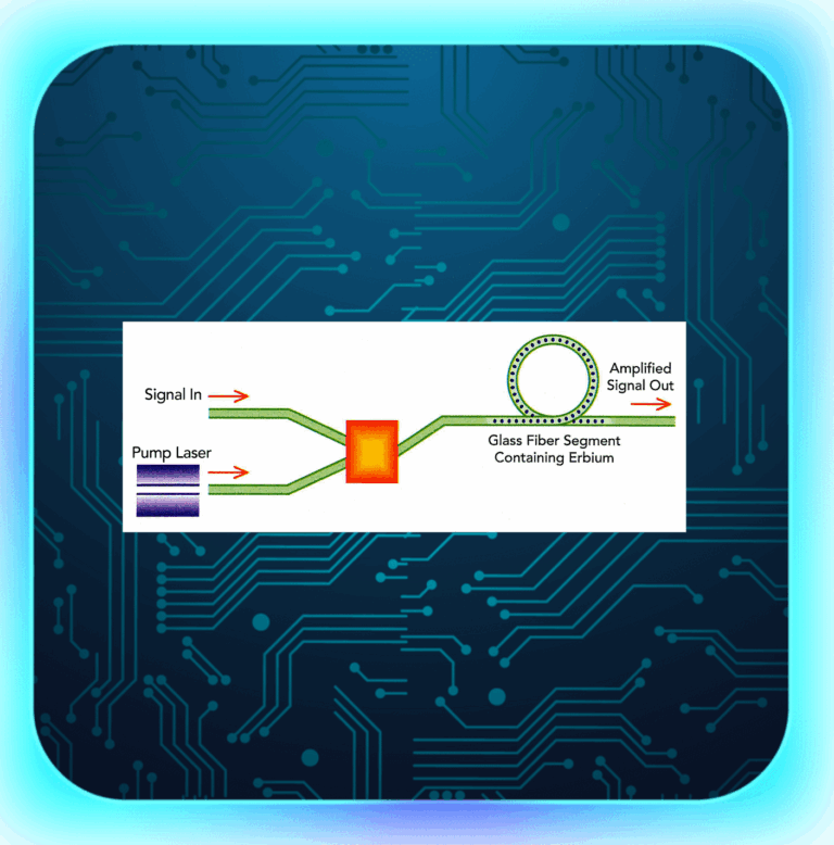
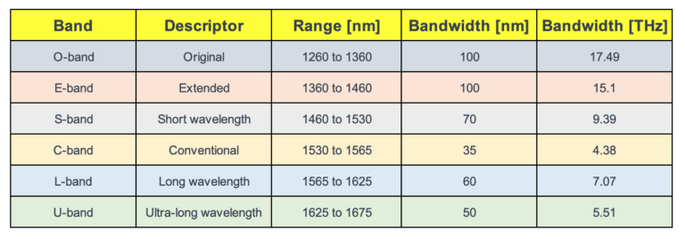
The main advantages and drawbacks of EDFAs are as follows.

Advantages

  • Commercially available in C band (1,530 to 1,565 nm) and L band (1,560 to 1,605) and up to  84-nm range at the laboratory stage.
  • Excellent coupling: The amplifier medium is an SM fiber;
  • Insensitivity to light polarization state;
  • Low sensitivity to temperature;
  • High gain: > 30 dB with gain flatness < ±0.8 dB and < ±0.5 dB in C and L band, respectively, in the scientific literature and in the manufacturer documentation
  • Low noise figure: 4.5 to 6 dB
  • No distortion at high bit rates;
  • Simultaneous amplification of wavelength division multiplexed signals;
  • Immunity to crosstalk among wavelength multiplexed channels (to a large extent)

Drawbacks

  • Pump laser necessary;
  • Difficult to integrate with other components;
  • Need to use a gain equalizer for multistage amplification;
  • Dropping channels can give rise to errors in surviving channels:dynamic control of amplifiers is  necessary.