MapYourTech · MapYourBasics Series
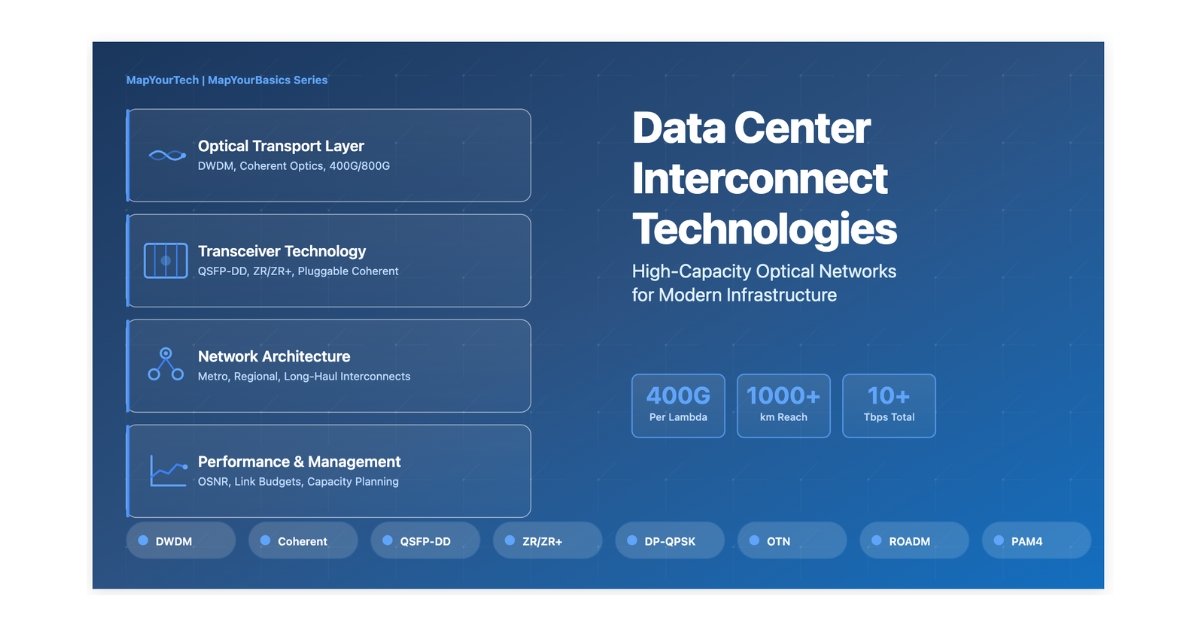
Data Center Interconnect (DCI) Technologies
From the capacity and power-budget math to coherent pluggables, the physical impairments that cap reach, the gray-versus-DWDM-versus-ZR decision, two calculators, and field case studies.
Introduction
Data Center Interconnect is the optical transport that links two or more data centers so they can replicate storage, migrate workloads, and fail over without losing state. It spans three distance regimes that each pull a different technology: intra-city and campus runs under a few kilometres on short-reach gray optics, metro links of 10 to 80 km on either passive DWDM or 400ZR-class coherent pluggables, and regional or long-haul routes beyond 500 km on full coherent line systems. This guide works through the capacity and power-budget math that decides what fits, the components and impairments behind those limits, the architecture choices an operator actually makes, and two calculators to run a budget and weigh the options.
The shape of the problem: DCI is a three-way trade among reach, capacity, and cost per bit. Short links want the cheapest optics that clear the span; long links want the spectral efficiency and DSP that only coherent provides; and the power-per-bit envelope of a pluggable decides whether it fits a router cage at all.
1. Fundamentals and Core Concepts
DCI carries high-capacity, low-latency optical transport between sites using wavelength division multiplexing, coherent optics, and pluggable modules from 100G to 800G and beyond. The business case is concrete: real-time replication between a primary and a backup site for disaster recovery, workload distribution to balance compute, geographic placement to cut user latency, and capacity growth by adding interconnected facilities rather than rebuilding one. Each driver translates to a number on the link budget — replication wants bounded latency, distribution wants aggregate capacity, and growth wants spare wavelengths.
| Distance | Application | Key requirement | Typical technology |
|---|---|---|---|
| Intra-city (< 10 km) | Campus, metro DCI | Latency < 50 µs, capacity | 100G/400G SR/DR/FR |
| Metro (10–80 km) | City-wide | Low latency, cost | 400G ZR-lite, DWDM |
| Regional (80–500 km) | Regional cloud, edge | Reach and capacity | 400G ZR, coherent DWDM |
| Long-haul (> 500 km) | Inter-regional | Maximum reach | 400G/800G ZR+, coherent |
The infrastructure stake is large: hyperscale clouds run DCI meshes linking hundreds of facilities, 5G cores and edge nodes depend on it for backhaul, and hybrid multi-cloud architectures rely on it for interconnection. A useful mental model is a road network — wider roads carry more traffic, shorter routes cut delay, and the topology decides how well the whole system uses its capacity.
2. Mathematical Framework
Shannon-Hartley capacity
C = B · log₂(1 + SNR)
Practical Example — capacity of a 50 GHz channel.
With B = 50 GHz and SNR = 25 dB (316 linear): C = 50×10⁹ · log₂(317) = 50×10⁹ × 8.31 ≈ 415 Gb/s. The headroom above 400G is why a 400G channel on a 50 GHz grid is comfortably inside the Shannon bound with a real coded modulation, not riding its edge.
Required OSNR by modulation (representative, 0.1 nm)
QPSK 12–15 dB · 8QAM 15–18 dB · 16QAM 22–26 dB · 64QAM 30+ dB
Each step up the constellation buys spectral efficiency and costs OSNR, which is why short links run dense formats and long links drop back to QPSK. Across an amplified chain OSNR adds reciprocally, 1/OSNRtotal = Σ 1/OSNRi.
Link power budget
PRX = PTX − αL − Σ(losses) + Gamp − M
Practical Example — 80 km metro, no amplifier.
PTX +2 dBm, α 0.22 dB/km, four connectors at 0.5 dB, 3 dB margin:
PRX = +2 − (0.22×80) − 2 − 3 = +2 − 17.6 − 2 − 3 = −20.6 dBm.
Against a −18 dBm direct-detect sensitivity this fails by 2.6 dB — the link needs an inline amplifier, a higher-power module, or a coherent receiver whose sensitivity sits well below −18 dBm. The same span is trivial for a coherent ZR module, which is exactly why metro DCI moved to coherent.
Chromatic dispersion accumulation
Dtotal = D · L · Δλ
At 17 ps/(nm·km) the tolerance scales as 1/B²: roughly 1200 ps/nm at 10G, 75 ps/nm at 40G, 12 ps/nm at 100G direct-detect. Coherent systems sidestep the limit entirely — DSP compensates dispersion digitally, which is the single biggest reason coherent replaced dispersion-managed line systems.
3. Types and Components
| Class | Distance | Speeds | Technologies |
|---|---|---|---|
| Intra-DC short reach | < 500 m | 100/400/800G | SR4, SR8, AOC, DAC |
| Campus / inter-building | 500 m – 2 km | 100/400G | DR4, FR4, PSM4 |
| Metro DCI | 2 – 80 km | 100/400G | ZR-lite, LR4, ER4, CWDM |
| Regional DCI | 80 – 500 km | 100/200/400G | ZR, coherent DWDM |
| Long-haul DCI | > 500 km | 100/400/800G | ZR+, DCO, coherent |
Transceivers
The module converts electrical to optical and back. QSFP-DD hosts 400G across SR8/DR4/FR4/ZR variants; OSFP adds thermal headroom for 800G; CFP2-DCO carries digital coherent for long-haul. The full pluggable family spans direct-detect short reach through coherent long-haul.
| Module | Speed | Reach | Modulation | Power |
|---|---|---|---|---|
| QSFP28 SR4 | 100G | 100 m | NRZ | 3.5 W |
| QSFP28 LR4 | 100G | 10 km | NRZ | 4.5 W |
| QSFP-DD DR4 | 400G | 500 m | PAM4 | 12 W |
| QSFP-DD FR4 | 400G | 2 km | PAM4 | 14 W |
| QSFP-DD ZR | 400G | 80–120 km | 16QAM coherent | 15–20 W |
| QSFP-DD ZR+ | 400G | ~1000 km | QPSK/8QAM adaptive | 15–22 W |
DWDM elements and coherent systems
A DWDM layer adds transponders or muxponders, passive or active mux/demux, EDFAs for span loss, and ROADMs for wavelength routing and add/drop — on a 50 GHz grid that is 80+ channels in the C-band, or flex-grid for super-channels. Coherent transmission multiplies it: polarization multiplexing doubles capacity, advanced modulation trades reach for spectral efficiency, and DSP compensates dispersion, PMD, and some nonlinearity. Coherent reaches 1000+ km against under 120 km for direct detection, at 2–8 bits/s/Hz versus 1–2, for 15–25 W versus 3–14 W.
| Format | Bits/symbol | Efficiency | Required OSNR | Reach |
|---|---|---|---|---|
| NRZ (OOK) | 1 | 1 b/s/Hz | ~15 dB | 80 km |
| PAM4 | 2 | 2 b/s/Hz | ~18 dB | 2–10 km |
| DP-QPSK | 4 | 2 b/s/Hz | 12–15 dB | 1000+ km |
| DP-8QAM | 6 | 3 b/s/Hz | 15–18 dB | 200–500 km |
| DP-16QAM | 8 | 4 b/s/Hz | 22–26 dB | 80–200 km |
| DP-64QAM | 12 | 6 b/s/Hz | 30+ dB | < 80 km |
4. Effects and Impacts
Four physical mechanisms degrade a DCI link. Fiber attenuation (0.2–0.25 dB/km at 1550 nm) sets the unamplified reach — 80 km at 10G, dropping to a few kilometres at 400G direct-detect, but 120 km on a coherent ZR. Chromatic dispersion (~17 ps/(nm·km)) broadens pulses and scales with the square of bit rate. PMD (0.01–0.5 ps/√km) randomly splits the polarizations and matters above 40G. And above a few dBm per channel the Kerr nonlinearities appear.
| Effect | Mechanism | Impact | Mitigation |
|---|---|---|---|
| SPM | Self-induced phase shift | Spectral broadening | Manage launch power |
| XPM | Phase shift from neighbours | Inter-channel interference | Spacing, power control |
| FWM | New mixing products | Crosstalk, depletion | Dispersion, uneven spacing |
| SRS | Power to longer wavelengths | Spectral tilt | Power shaping |
| SBS | Backward scattering | Caps launch near ~10 dBm | Linewidth broadening |
| Metric | Excellent | Good | Marginal | Poor |
|---|---|---|---|---|
| BER | < 10-15 | 10-12–10-15 | 10-9–10-12 | > 10-9 |
| OSNR (100G QPSK) | > 20 dB | 15–20 dB | 12–15 dB | < 12 dB |
| Q-factor | > 15 dB | 10–15 dB | 7–10 dB | < 7 dB |
Power efficiency improves with rate: a 10G SFP+ burns ~1 W (0.1 W/Gb/s); 100G QSFP28 ~4 W (0.04); 400G QSFP-DD ~12–15 W (0.03–0.04); a 400G coherent ZR ~18 W (0.045) — slightly higher per bit, but it buys the reach a direct-detect module cannot reach.
5. Techniques and Solutions
Four implementation models, in rising order of reach and cost. Gray optics use standard client transceivers, cheapest and simplest but one wavelength per fiber and under ~10 km — good for intra-DC and campus. DWDM with external transponders gives the most wavelengths (40–80+) and full protocol flexibility at the highest capital cost and complexity — the carrier choice. Pluggable colored DWDM puts the wavelength in the module, eliminating the transponder shelf for moderate channel counts. Coherent pluggables (ZR/ZR+/DCO) carry the longest reach at the highest per-port cost and power, and underpin the IP-over-DWDM model where the wavelength lives in the router line card.
| Criterion | Gray optics | DWDM + transponders | Pluggable DWDM | Coherent pluggables |
|---|---|---|---|---|
| Max distance | 2–10 km | 80–2000 km | 40–120 km | 120–1000+ km |
| Capacity/fiber | 100–400G | 4–40+ Tb/s | 1–8 Tb/s | 400–800G/λ |
| Cost/port | $500–2K | $10K–50K | $3K–10K | $15K–40K |
| Power/100G | 4 W | 15–25 W | 4–6 W | 15–20 W |
| Flexibility | Low | Very high | Medium | High |
Forward error correction
RS-FEC adds ~7% overhead for ~5 dB coding gain in 100G/400G; soft-decision FEC adds 20–25% for up to 11 dB in coherent systems. SD-FEC is what stretches a 400G ZR+ link from roughly 500 km to 1000+ km by correcting errors that would otherwise drop the link — the OIF 400ZR and 800ZR pluggables use concatenated and open FEC variants.
Dispersion management and protection
Coherent DSP compensates dispersion across an effectively unlimited range, displacing DCF modules and chirped gratings on new builds. For availability, optical 1+1 switches under 5 ms, SONET/SDH rings and MPLS fast-reroute under 50 ms; modern IPoDWDM designs increasingly handle protection at the IP layer with ECMP across diverse paths.
6. Design Methodology
Work in four phases. Define requirements — capacity now and on a 3–5 year forecast, distance and fiber quality, availability target, and the cost and power budget. Select technology against distance and capacity. Build the power budget. Then verify OSNR for amplified routes.
| Distance | Capacity | Consider | With |
|---|---|---|---|
| < 500 m | 100–400G | SR/DR + MMF | AOC for flexibility |
| 0.5–2 km | 100–400G | DR4/FR4 + SMF | PSM4 for cost |
| 2–40 km | < 1 Tb/s | LR4/ER4 gray | CWDM |
| 10–80 km | > 1 Tb/s | DWDM colored | Passive mux/demux |
| 80–500 km | High | 400G ZR coherent | ROADM |
| > 500 km | Maximum | ZR+ with SD-FEC | Full DWDM platform |
Practical Example — 400G ZR-lite over 80 km, worksheet.
PTX +2 dBm; fiber 80×0.22 = −17.6 dB; six connectors −3.0 dB; two splices −0.2 dB; mux/demux −3.0 dB; margin −3.0 dB → total −26.8 dB → PRX = −24.8 dBm. Against a −26 dBm coherent sensitivity that is +1.2 dB of headroom — it runs, but with almost nothing in reserve, so either raise launch power or add an inline amplifier before committing.
For amplified routes verify OSNR with the engineering form — OSNRspan = 58 + Pch − Lspan − NF, then subtract 10·log(N) for N spans; the +58 carries the 0.1 nm reference, so never subtract a bandwidth term again. A 400G 16QAM channel wants about 22 dB at the receiver. An unamplified 80 km metro span has no EDFA ASE, so OSNR there is set by transmitter and receiver noise and typically exceeds 30 dB.
Pitfalls: skip the 3–5 dB margin and the link fails as it ages; push launch past ~5 dBm/channel and FWM and XPM dominate; run high-rate formats on legacy high-PMD fiber and the DSP cannot keep up; undersize cooling and 400G modules throttle; ignore the ~5 µs/km propagation delay on latency-sensitive routes; and single-path anything that needs five-nines.
7. Interactive Calculators
Two tools: a link-budget calculator that breaks the loss down and tests it against receiver sensitivity, and a heuristic technology-fit scorer that weighs five DCI options against a distance, capacity, and cost-versus-performance priority. The second is a planning aid — it ranks options, it does not replace the budget the first one computes.
8. Applications and Case Studies
Practical Example — hyperscale regional ring.
Five sites across a 150 km metro, 10 Tb/s growing to 40 Tb/s, five-nines. Built on 400G ZR coherent QSFP-DD over a 50 GHz DWDM ring with 1+1 optical protection: 32 wavelengths give 12.8 Tb/s with C+L headroom to 40 Tb/s. The longest 85 km span held OSNR above 25 dB (ample for 16QAM), round-trip latency stayed near 0.75 ms, and putting the coherent optics in the switch rather than a transponder shelf cut both the per-100G cost and the deployment time sharply.
Practical Example — low-latency trading link.
A 12 km exchange interconnect with a sub-60 µs one-way budget ran 400G DR4 over dedicated dark fiber on the shortest physical route, hitting about 58 µs of pure propagation delay with dual diverse paths and sub-microsecond optical switching. Here the constraint is geometry, not the optical budget — every metre of fiber is ~5 ns, so route length, not modulation, is the design variable.
Practical Example — global multi-site DR.
Twelve sites across 200–3500 km mixed 400G ZR intra-region with 100G/200G ZR+ inter-region (to ~2000 km) and OTN switching for grooming and protection, aggregating near 9.8 Tb/s. The mixed-reach mesh is the realistic enterprise pattern: dense formats where spans are short, QPSK-class where they are long, and a mixed-rate line plan holding it together.
| Symptom | Likely cause | Fix |
|---|---|---|
| High BER / loss | Low OSNR, dispersion, dirty connector | Check OSNR, clean connectors, add amplification |
| Link flapping | Marginal power, temperature | Raise margin, secure connections |
| Cannot hit line rate | FEC or protocol overhead | Check FEC mode and frame size |
| Intermittent errors | PMD, fiber stress | Low-PMD fiber, relieve stress, go coherent |
| Wavelength drift | Laser temperature | Improve cooling, check grid alignment |
| Application | Distance | Solution | Cost/100G |
|---|---|---|---|
| Intra-DC | < 500 m | SR/DR + MMF or AOC | $300–1K |
| Campus | 0.5–2 km | DR4/FR4 + SMF | $1–2K |
| Metro (low density) | 2–40 km | LR4/ER4 gray | $2–3K |
| Metro (high density) | 10–80 km | DWDM colored + mux | $3–5K |
| Regional | 80–500 km | 400G ZR + ROADM | $10–15K |
| Long-haul | > 500 km | ZR+/DCO with SD-FEC | $15–30K |
Main Points
References
- Optical Internetworking Forum, Implementation Agreement OIF-400ZR — 400G Coherent DWDM for DCI Applications, OIF.
- ITU-T, Spectral grids for WDM applications: DWDM frequency grid (G.694.1), ITU-T Study Group 15.
- IEEE, Standard for Ethernet (IEEE 802.3) — 100G, 400G, and 800G physical layer specifications, IEEE.
Sanjay Yadav, "Optical Network Communications: An Engineer's Perspective" — Bridge the Gap Between Theory and Practice in Optical Networking.
Developed by MapYourTech Team
For educational purposes in Optical Networking Communications Technologies
Note: This guide is based on industry standards, best practices, and real-world implementation experiences. Specific implementations may vary based on equipment vendors, network topology, and regulatory requirements. Always consult with qualified network engineers and follow vendor documentation for actual deployments.
Feedback Welcome: If you have any suggestions, corrections, or improvements to propose, please feel free to write to us at [email protected]

Optical Communications & Network Automation Expert | Author of 3 Books for Optical Engineers | Founder, MapYourTech
Optical networking engineer with nearly two decades of experience across DWDM, OTN, coherent optics, submarine systems, and cloud infrastructure. Founder of MapYourTech. Read full bio →
Follow on LinkedInRelated Articles on MapYourTech