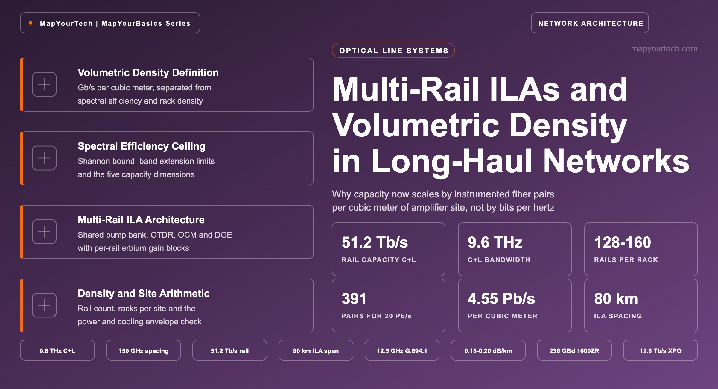
Multi-Rail Architectures and Volumetric Density in Long-Haul Networks
Why the industry stopped optimising bits per hertz and started counting instrumented fiber pairs per cubic meter of amplifier site.
Capacity per hertz has a ceiling; capacity per cubic meter is still an engineering choice.
What You Will Learn
- Define volumetric density as Gb/s per cubic meter and separate it from spectral efficiency, rack density and capacity per fiber pair (Section 2, Figure 1).
- Compute a rail capacity of 51.2 Tb/s from 9.6 THz of C+L spectrum at 150 GHz spacing with 800 Gb/s carriers (Section 3).
- Trace which subsystems a multi-rail in-line amplifier shares — pump bank, OTDR, OCM, DGE, OSC — and which stay per rail (Section 4, Figures 3 and 4).
- Convert a 20 Pb/s route requirement into 391 fiber pairs, 4 racks of amplification and 12 intermediate sites on a 1,000 km route (Section 5).
- Quantify the shared-hardware ratio and read the widened failure domain it produces against a per-pair reference (Sections 5 and 6).
- Sequence a staged rail turn-up so that amplifier calibration holds from rail 1 to rail 128 without a re-optimisation window (Section 7, Figure 6).
- Separate a per-rail defect from a shared-subsystem defect using OTDR scheduling, OCM dwell time and alarm correlation (Sections 8 and 9).
- Select between a conventional per-pair line system, a multi-rail platform and new cable plant using the decision criteria of Section 10.
1Introduction
An in-line amplifier hut on a long-haul route holds a fixed number of racks, draws a fixed power feed, and runs a cooling plant sized when the building was commissioned. None of those three quantities changes when the traffic between two data centers grows from four fiber pairs to two hundred. That mismatch — between a capacity requirement that is scaling with distributed compute and a physical envelope that was poured in concrete decades ago — is the constraint that reorganised optical line system design during 2026.
The pressure has a specific origin. AI training and inference workloads no longer fit inside one building, so operators interconnect campuses and regions at capacities that used to describe an entire national core network. A hyperscale operator presented at OFC 2026 that regional data center interconnection has typically needed 16 to 48 fiber pairs, while AI-driven regional interconnection needs 128 or more (operator statement). An industry analyst reported discussions at the same event pointing to 20 Pb/s between the back ends of two GPU data centers, which converts to roughly 390 fiber pairs when each pair is filled with 800 Gb/s pluggable coherent optics (analyst assessment). Wavelength-by-wavelength growth does not reach those numbers, and neither does fiber-by-fiber growth using one conventional line system per pair.
Scope and Boundary Conditions
This article covers terrestrial long-haul and regional line systems built from erbium-doped fiber amplifiers and coherent transponders, in the range where in-line amplification is required — roughly 80 km per span and above. It works through the volumetric density metric, the multi-rail in-line amplifier architecture that produces it, the arithmetic that sizes a deployment, and the operational consequences of sharing instrumentation across rails. It does not cover intra-data-center optics, co-packaged optics for scale-up fabrics, or submarine wet plant, each of which has a different physical envelope and a different cost structure.
Four suppliers put multi-rail products into the public record during 2026 — Ciena, Cisco, Coherent Corp. and Nokia — and three more were reported to be evaluating systems of their own, with commercial shipments assessed as likely to begin during 2027 (analyst assessment). One supplier markets its platform under the hyper-rail name and states that hyper-rail is sometimes called multi-rail; analyst and trade coverage has settled on multi-rail as the generic term, and this article follows that usage. Rail-count claims differ between suppliers and are quoted here with attribution rather than compared as a ranking, because the configurations behind them differ in band coverage, chassis depth and power feed.
The reader who wants the underlying transmission physics before the architecture will find the capacity bound treated in the MapYourTech guide to Shannon's limits for fiber optics, and the band mechanics in the treatment of C-band, L-band and C+L band DWDM.
Takeaway: the binding constraint on a long-haul capacity upgrade has moved from the spectrum inside a fiber to the volume, power and cooling available at the sites that amplify it.
2Volumetric Density Definition and Component Terms
Volumetric density is the carried capacity a line system delivers per unit of physical volume it occupies at a site, stated in gigabits per second per cubic meter. It counts the equipment volume of the terminal or amplifier hardware, including the rack envelope that hardware requires, and it divides the summed capacity of every fiber pair that hardware serves by that volume. Spectral efficiency does not appear in it.
Distinctions From Adjacent Quantities
Four quantities get conflated with volumetric density and each answers a different question. Spectral efficiency, in bits per second per hertz, measures how much information a modem extracts from a given slice of spectrum and is bounded by the transmission physics of the fiber. Capacity per fiber pair, in terabits per second, is spectral efficiency multiplied by the amplified bandwidth, and it stops rising when both terms stop rising. Rack density, in rails per rack or per rack unit, is a packaging count with no capacity term in it, so it compares two platforms only when their per-rail capacities match. Power density, in watts per rail or watts per terabit, is the constraint that usually binds first in an older hut, and it is independent of volume: a rack that fits the floor may still exceed the feed.
Volumetric density folds capacity and packaging into one number and deliberately leaves power out, which is its main limitation as a planning metric. A platform can improve volumetric density while leaving the site power draw unchanged, and in an amplifier hut where a large fraction of the feed already goes to cooling, that improvement delivers nothing. Both numbers are needed, and Section 6 treats them together.
Units and Conversion
Dv = (Nrails × Crail) / V [Gb/s·m−3]
Where:
- Dv — volumetric density, Gb/s per cubic meter. Typical values computed in this article fall between 1 × 10⁶ and 5 × 10⁶ Gb/s/m3 for C+L amplification.
- Nrails — number of instrumented fiber pairs the hardware in that volume serves. Vendor-stated figures for announced multi-rail platforms range from 128 to 160 per rack.
- Crail — filled capacity of one rail, Gb/s. 51,200 Gb/s for a 9.6 THz C+L allocation at 150 GHz spacing with 800 Gb/s carriers.
- V — external volume of the equipment envelope, m3. 1.44 m3 for a nominal 600 mm × 1200 mm × 2000 mm cabinet.
Practical Example — volumetric density of one multi-rail amplifier rack
Take a rack of C+L multi-rail in-line amplifiers stated by its supplier to carry 128 rails (vendor claim). Each rail carries the 9.6 THz C+L allocation at 150 GHz spacing, which gives 9,600 ÷ 150 = 64 carriers per direction; at 800 Gb/s per carrier the rail capacity is 64 × 800 = 51,200 Gb/s. The rack therefore serves 128 × 51,200 = 6,553,600 Gb/s, or 6.55 Pb/s. Dividing by the 1.44 m3 cabinet envelope gives Dv = 4,551,111 Gb/s/m3, which rounds to 4.55 Pb/s per cubic meter. Swap the 800 Gb/s carrier for a 1.2 Tb/s embedded engine on the same grid and Crail rises to 76.8 Tb/s, lifting Dv to 6.83 Pb/s/m3 with no change to the amplifier at all — which is the point of separating the two terms.
Takeaway: volumetric density is a ratio with a capacity numerator and a site-planning denominator, so a platform improves it either by raising per-rail capacity or by shrinking the volume that serves a rail — and the two levers are independent.
3Spectral Efficiency Ceiling and Capacity Scaling Dimensions
Fiber capacity has five physical dimensions available to it — time, quadrature, polarization, frequency and space — and four of them are close to exhausted in commercial long-haul systems. Symbol rate has been rising at roughly ten percent per year, limited by the converter technology in the coherent digital signal processor rather than by the fiber. Quadrature and polarization are fully used by dual-polarization coherent modulation. Frequency has been extended from the C-band into the L-band and then into the widened super-C and super-L variants. Space, meaning additional fiber pairs, is the dimension that remains.
Complete Capacity Bound
C = 2 · B · log2(1 + SNR) [bit/s]
Where:
- C — channel capacity in bits per second (theoretical limit).
- B — bandwidth in hertz, equal to the symbol rate Rs for a matched root-raised-cosine filter. Deployed coherent carriers run between about 60 GBd and 140 GBd, with 236 GBd targeted for the 1600ZR generation.
- SNR — signal-to-noise ratio in the signal bandwidth, linear. Long-haul operating points fall between roughly 8 dB and 18 dB.
- 2 — the two orthogonal polarization states, the only two that exist.
Per-symbol spectral efficiency follows as C/B = 2 · log2(1 + SNR) in bit/s/Hz, and the occupied bandwidth that sets channel spacing is a separate quantity, Bocc = Rs(1 + β), where β is the pulse-shaping roll-off.
The logarithm is the whole difficulty. Doubling capacity at a fixed reach requires squaring the signal-to-noise ratio, while doubling reach at fixed capacity costs about 3 dB. Textbook treatments of capacity scaling put the correct system metric at 2SE × L rather than the older capacity-distance product, precisely because spectral efficiency enters the relation logarithmically and distance enters linearly (published analysis). Modern probabilistically shaped coherent modems already operate within roughly 0.1 dB to 1 dB of the linear additive-white-Gaussian-noise bound at their operating point, so the remaining engineering headroom in the modulation dimension is small.
Above the linear bound sits the nonlinear one. Launch power raises the linear signal-to-noise ratio until Kerr-effect nonlinear interference rises faster, and the resulting capacity curve has a maximum at an optimum launch power rather than growing without bound. Under the Gaussian Noise model the effective signal-to-noise ratio at that optimum sits 1.76 dB below the linear value, which fixes a finite practical capacity for a given link (model-derived bound). The information-theoretic literature is careful that this is a lower bound on the true channel capacity rather than a proven ceiling, and the question of whether the real fiber channel has a finite capacity at high power remains open. For a planner the distinction does not change the design: no deployed or announced modem generation moves the number enough to reduce the fiber-pair count for a petabit-class route. The interaction between launch power and nonlinear penalty is worked through in detail in the MapYourTech reference on OSNR, GOSNR and launch power optimisation, and readers can run the capacity relation directly in the Shannon Limit Calculator.
| Dimension | Mechanism | Recent scaling | Binding constraint |
|---|---|---|---|
| Time (symbol rate) | More symbols per second per carrier | ~10% / year | Converter bandwidth and power in the coherent DSP |
| Quadrature | In-phase and quadrature components | Fully used | Two components exist and both are in use |
| Polarization | Two orthogonal states multiplexed | Fully used | Two states exist and both are in use |
| Modulation order | More bits per symbol | ~0.1–1 dB gap | Logarithmic return against required SNR; reach falls |
| Frequency (band) | C-band to C+L to super-C and super-L | 9.6–12 THz | Amplifier gain bandwidth; band-splitter loss and guard band |
| Space (fiber pairs) | Parallel instrumented fiber pairs | Unbounded | Volume, power and cooling at every amplifier site |
Band Extension and Its Diminishing Return
Spectrum extension has been the workhorse of the last decade because it scales capacity roughly linearly with the cost of one additional amplifier band on already-installed fiber. Vendors converged on a symmetric arrangement of about 4.8 THz of C-band and 4.8 THz of L-band for a conventional 9.6 THz system, and pushing erbium designs to their edges yields super-C and super-L bands of about 6 THz each for roughly 12 THz total (industry practice). That is an increase of 20% to 30% over the earlier arrangement, and it comes with four recurring penalties: band-splitter and combiner insertion loss at every amplifier site, an inter-band gap that no channel occupies, higher L-band amplifier noise figure, and inter-channel stimulated Raman scattering that transfers power from the shorter wavelengths to the longer ones across the whole occupied band. The resulting generalized signal-to-noise ratio gradient across a loaded C+L system reaches 3.5 dB or more and is treated as a permanent design input. The mechanics are covered in the MapYourTech articles on band allocation strategy in C+L network design and inter-band Raman transfer in loaded C+L systems, and the tilt can be visualised for a specific loading in the C+L Band SRS Visualiser.
What remains after both levers is arithmetic. A route requirement stated in petabits divided by a per-pair capacity in tens of terabits gives a fiber-pair count in the hundreds, and that count is the input to every site-level decision that follows.
| Route capacity | Pairs at 51.2 Tb/s | Pairs at 76.8 Tb/s |
|---|---|---|
| 2 Pb/s | 40 | 27 |
| 5 Pb/s | 98 | 66 |
| 10 Pb/s | 196 | 131 |
| 20 Pb/s | 391 | 261 |
| 40 Pb/s | 782 | 521 |
Takeaway: modulation and band extension together move the per-pair capacity by tens of percent, while AI-driven route requirements have moved by factors of ten, so the fiber-pair count rather than the spectral efficiency sets the equipment problem.
4Multi-Rail Line System Architecture
A multi-rail line system integrates the transmission infrastructure of N parallel fiber pairs into one managed platform and shares selected hardware across all N rails rather than replicating it per rail. Each rail remains an independent optical path with its own amplification and its own spectrum; what changes is that the instrumentation, the pump energy source, the equalisation engine and the control processor serve the whole group.
Conventional Per-Pair Reference
A conventional in-line amplifier site carries one line system per fiber pair. Each system holds a pre-amplifier and a booster, a gain-flattening filter, a variable optical attenuator for gain control, an optical supervisory channel transceiver on a dedicated wavelength, an optical channel monitor for per-channel power readings, a reflectometer for fiber characterisation, and in a C+L system a band splitter and combiner with a second amplifier chain. Every one of those functions is replicated when a second fiber pair is lit. Cost per terahertz and power per terahertz therefore scale linearly with the number of pairs, and so does the rack space.
What Gets Shared and Why It Can Be
Four elements dominate the integration. The first is the pump laser. Multi-rail designs use uncooled and multi-chip pump lasers, which removes the thermoelectric cooler and its control loop from each pump assembly and allows one pump bank to feed erbium gain blocks on several rails. Removing the cooler is where a large part of the power reduction comes from, and it also removes a component with a well-known wear-out mechanism. The second is the reflectometer. A fiber characterisation measurement is intermittent by nature — a route is tested at turn-up and then on demand or on a schedule — so one reflectometer behind an optical switch can serve many rails without any rail losing a capability it used continuously.
The third is the optical channel monitor. Per-channel power readings are a sampled measurement, and a monitor stepping through rails on a cycle delivers the same information at a longer refresh interval. The fourth is dynamic gain equalisation. A gain equaliser corrects the spectral shape a rail acquires from amplifier ripple and Raman tilt, and because the correction changes slowly, one engine with per-rail filter paths can hold several rails flat. Section 8 covers what the longer refresh intervals cost in practice.
| Subsystem | Placement | Reason | Rails affected by one defect |
|---|---|---|---|
| Erbium gain block | Per rail | Carries the signal; cannot be time-shared | One |
| Gain-flattening filter | Per rail | Fixed spectral shape in the signal path | One |
| Variable optical attenuator | Per rail | Sets per-rail gain and tilt continuously | One |
| Pump laser bank | Shared | Uncooled multi-chip pumps feed several coils | All in the group |
| Reflectometer (OTDR) | Shared | Measurement is intermittent and scheduled | Loss of test access only |
| Channel monitor (OCM) | Shared | Sampled measurement behind a rail-select switch | Loss of visibility only |
| Gain equaliser (DGE) | Shared engine, per-rail paths | Correction changes slowly | Equalisation for all in the group |
| Supervisory channel (OSC) | Shared or per rail by design | Depends on whether rails share a cable route | Design-dependent |
| Control processor | Shared | One managed entity per platform | All in the group |
| Power feed and cooling | Shared | One chassis, one feed | All in the group |
Takeaway: multi-rail integration pools the intermittent and the slow functions and leaves the continuous signal-path functions per rail, which is why the ratio of managed hardware to rails can fall below one without changing the optical performance of any individual rail.
5Density, Capacity and Power Arithmetic
Sizing a multi-rail deployment runs in five steps: convert the route capacity requirement into a fiber-pair count, convert the pair count into racks at each amplifier site, count the sites along the route, check the power feed, and check the cooling. Each step has a closed-form relation and only the last two commonly fail.
Rail Capacity From Spectrum and Spacing
Crail = ⌊Btotal / Δf⌋ × Rnet [Gb/s]
Where:
- Btotal — amplified bandwidth per direction, GHz. 9,600 GHz for a conventional C+L system; about 12,000 GHz for super-C plus super-L (industry practice).
- Δf — channel spacing, GHz. 150 GHz suits an 800 Gb/s carrier at present symbol rates; the slot must be a multiple of 12.5 GHz per ITU-T G.694.1.
- Rnet — net client rate per carrier, Gb/s. 800 Gb/s for a ZR-class pluggable; 1,200 Gb/s for a current embedded engine.
Worked: ⌊9,600 / 150⌋ = 64 carriers; 64 × 800 = 51,200 Gb/s = 51.2 Tb/s per rail.
Shared-Hardware Ratio
ρ = Hshared / Nrails [instances per rail]
Where:
- Hshared — count of a given managed hardware type in the platform: reflectometers, channel monitors, gain-equaliser engines, control processors.
- Nrails — rails the platform serves.
- ρ — instances per rail. A conventional line system has ρ = 1 for every type. A platform with one reflectometer across 16 rails has ρ = 0.0625.
The ratio crossing below 1:1 is the architectural change; the specific value is a product decision that differs between suppliers.
Site Count and Amplifier Racks
Rsite = ⌈Npairs / Nrack⌉ and S = ⌈Lroute / Lspan⌉ − 1
Where:
- Npairs — fiber pairs the route requires, from route capacity divided by Crail.
- Nrack — rails a rack of multi-rail amplifiers serves. 128 and 160 are vendor-stated figures for announced platforms.
- Lroute — route length in km; Lspan — amplifier spacing, typically 80 km on terrestrial long-haul plant.
- S — intermediate amplifier sites, excluding the two terminals.
Practical Example — sizing a 20 Pb/s scale-across route over 1,000 km
Start from the route requirement of 20 Pb/s discussed at OFC 2026 for connecting the back ends of two GPU data centers (analyst assessment). Dividing 20,000 Tb/s by the 51.2 Tb/s rail capacity computed above gives 390.6, so the route needs 391 fiber pairs. At a vendor-stated 128 rails per rack, Rsite = ⌈391 / 128⌉ = 4 racks of in-line amplification at every intermediate site. On a 1,000 km route at 80 km spacing, S = ⌈1,000 / 80⌉ − 1 = 12 intermediate sites, so the deployment places 48 amplifier racks along the route in addition to the terminal equipment.
The same 391 pairs served by conventional per-pair line systems would need a rack count several times higher at every one of those 12 sites, which is the arithmetic that made the architecture necessary rather than merely attractive: most existing amplifier huts do not have the floor space, and a new building on an existing right of way is a multi-year project. Switching the carrier to a 1.2 Tb/s embedded engine on the same 150 GHz grid raises Crail to 76.8 Tb/s and drops the pair count to 261, which is 3 racks per site rather than 4 — a real saving, and still two orders of magnitude away from the pair counts these routes carried five years ago.
| Configuration | Rails per rack | Racks for 391 rails | Evidence class |
|---|---|---|---|
| Conventional per-pair baseline | 32 | 13 | Derived from analyst statement |
| Multi-rail platform, 128 rails | 128 | 4 | Vendor claim |
| Multi-rail platform, 160 rails | 160 | 3 | Vendor claim |
Power and Cooling Check
The volume calculation is the easy half. An amplifier hut has a fixed power feed and a cooling plant sized to the heat load the building was designed for, and one supplier states that in some cases as much as 70% of site power is consumed by cooling equipment (vendor statement). That figure sets the multiplier: a watt removed from the equipment removes more than a watt from the site draw, because it also removes the cooling load that served it. Uncooled pump lasers are the main contributor, and one supplier claims up to 75% power savings for its multi-rail platform against its own previous generation (vendor claim). Suppliers state power reductions against their own baselines rather than against a common reference, so these figures indicate the direction of the change rather than a comparison between platforms.
Design rule: size the site against the feed and the cooling plant before the floor plan. A rack count that fits the building and exceeds the feed is a deployment that stops at the rail where the breaker trips, and a hut retrofit for power and airflow has a longer lead time than the line system it hosts.
Takeaway: a route requirement in petabits converts to a pair count through one division, to a rack count through one more, and to a site programme through the span plan — and that rack count is only deliverable if the power feed and the cooling plant at each of those sites can carry it.
6Design Considerations and Trade-Offs
Three decisions dominate a multi-rail design: how many rails to place behind one shared subsystem, whether the rails on a platform may share a cable route, and how the group is placed relative to the protection and restoration scheme running above it. Each trades density against exposure.
Group Size and Correlated Exposure
Every rail added behind a shared pump bank or control processor increases the capacity that one defect can affect. A conventional per-pair architecture has no correlated failure mode at the amplifier: a pump failure removes one fiber pair. A platform sharing one pump bank across four rails removes four fiber pairs, which at 51.2 Tb/s each is 204.8 Tb/s from one component. That exposure is manageable and it is not new in kind — a shared power feed already correlates a whole bay — but it is new in degree, and it has to be declared to the layer that restores traffic.
The practical response is to treat the shared group as a shared risk link group in the routing layer. Two rails that must survive the same event belong on different platforms, ideally in different bays on different feeds, and preferably on different cable routes. That constraint costs density directly: a design that reserves half the rails on each platform for a diverse partner has half the effective rails per rack it advertises. The alternative is to accept the correlation and restore at the IP layer across the surviving rails, which works where the aggregate has enough spare capacity and fails where it does not. The trade-off between optical protection and higher-layer restoration is treated in the MapYourTech material on optimisation levers for C, L and C+L optical networks, and availability under a given fiber cut rate is modelled from the cut rate, the repair time and the diversity of the surviving paths.
Placing a working rail and its protecting rail behind the same shared pump bank removes the protection entirely while leaving every alarm and every management view reporting a healthy 1+1 pair. The optical paths are independent and the monitoring is independent, so nothing in the system reports the coupling; it exists only in the pump bank and the power feed. Record the shared group as a shared risk link group at design time, and validate it by inspection of the physical build rather than from the network management inventory.
Cable Route and Supervisory Channel
Rails on one platform may or may not share a cable. Where they do, a duct cut removes all of them at once and the shared supervisory channel is adequate because there is no case in which one rail is up and another down for a route reason. Where they do not, the supervisory channel has to be per rail or per cable route, because a shared channel would report the state of one route while carrying traffic on several. This is the design point that most often forces a per-rail element where the platform would otherwise share one, and it is worth settling before the platform is ordered rather than after.
Pump Supply and Component Lead Time
Uncooled multi-chip pump lasers come from a small number of manufacturers, so pump availability rather than card design can set how fast a multi-rail deployment proceeds. A deployment programme that assumes rack-rate delivery of 12 sites in parallel should confirm the component lead time before the site works are scheduled, because civil and power work booked against a delivery date carries a rescheduling cost measured in weeks.
Amplifier Calibration Under Partial Fill
A rail turned up empty and filled later presents its amplifier chain with a changing total load, and the control loops that hold gain and tilt were calibrated against one occupancy. The established answer is amplified spontaneous emission loading: shaped noise fills the unused spectrum so the amplifier chain sees a constant total load from day one, which keeps per-channel performance the same at first light as at full fill. The mechanism and its migration consequences are covered in the MapYourTech treatment of hitless C-band to C+L capacity migration. In a multi-rail context this matters more than it does per pair, because the number of turn-up events per site is now counted in hundreds and a re-optimisation window per rail is not available.
Takeaway: group size is the single design variable that sets both the density gained and the capacity a shared component can remove, so it is decided by the restoration scheme above the line system rather than by the amplifier data sheet.
7Implementation and Turn-Up Guidelines
A multi-rail deployment turns up hundreds of fiber pairs at each of a dozen sites, so the procedure that worked for four pairs does not survive contact with 391. Two properties have to hold: every step is scripted and repeatable, and no step requires a traffic-affecting window on a rail that is already carrying service.
Fiber Characterisation Before Amplification
Every rail is characterised before it is amplified. The reflectometer measures span loss, splice and connector events, and the distance to each, and the result is compared against the design span loss used in the link budget. A shared reflectometer means this runs as a sequence rather than in parallel, so the site plan should allow for the serial measurement time across the rails on each platform. Where the measured loss exceeds the design value the correct action is to fix the plant, not to raise launch power, because the additional power buys linear signal-to-noise ratio at the cost of nonlinear interference and the exchange is unfavourable above the optimum. Traces can be practised against known event patterns in the MapYourOTDR Simulator & Viewer.
Calibration at Full Occupancy
The amplifier chain on each rail is calibrated with the spectrum full, using channel loading to occupy every slot that will eventually carry a carrier. Calibrating at partial fill and expanding later requires a re-optimisation that in-service traffic will not permit, and at 128 rails per rack the accumulated cost of getting this wrong is a maintenance programme rather than a maintenance window.
Staged Rail Activation
Rails are activated in a fixed order and each activation is verified before the next begins. The sequence per rail is: characterise the fiber, install and inventory the card, load the design parameters from the planning tool, apply channel loading to full occupancy, calibrate gain and tilt, verify per-channel power against the design profile at the shared channel monitor, then hand the rail to service provisioning. Recording the post-calibration channel monitor profile as the rail baseline is the step teams most often omit at turn-up, and it is the reference every later fault comparison needs. The commissioning sequence and its acceptance criteria belong in a written method of procedure that every site team runs unchanged.
Integration With Installed Plant
A multi-rail platform placed into an existing route interoperates with whatever is already there, and the interoperation happens at the optical interface rather than in the management plane. The parameters to agree before installation are the per-channel launch power and its spectral density envelope, the band edges and any inter-band gap, the loading rules that apply when a carrier fails, and the monitoring access that has to keep working whether or not traffic is present. Where an existing route already carries conventional per-pair systems, adding a multi-rail platform on new pairs in the same cable changes the Raman interaction seen by the installed pairs only if the cable's total launched power changes materially, which it does when many new pairs are lit at once.
Takeaway: at 391 rails a turn-up procedure is a production line rather than a task list, and the two steps that make it repeatable are calibrating every rail at full occupancy and recording a channel monitor baseline before the rail carries service.
8Performance Monitoring and Shared-Instrument Constraints
Sharing an instrument across rails changes what the instrument can observe, and the change is in time rather than in accuracy. A channel monitor stepping through 16 rails delivers each rail's spectrum at one sixteenth of the rate it would achieve dedicated, so a transient that a dedicated monitor would catch may fall between visits. That trade is acceptable for the measurements the monitor is used for and unacceptable for a few, and separating the two is the monitoring design task.
What Survives Sampling and What Does Not
Slow observables survive. Per-channel power drift, amplifier gain ripple, accumulated tilt, filter narrowing across a cascade and the gradual rise in span loss that precedes a plant defect all change over hours to months, and a monitor visiting each rail every few minutes captures them with no loss of engineering value. Fast observables do not survive. A power transient during a protection switch, the gain excursion following a sudden channel loss, and the short-lived spectral shape during a control-loop settling event are all missed by a sampled monitor, and any procedure that depended on catching them has to move to a per-rail measurement in the transponder.
That relocation is usually available and often better. A coherent receiver estimates every impairment it corrects and reports most of them: chromatic dispersion, differential group delay, polarization-dependent loss, received power, pre-forward-error-correction bit error rate and an estimated signal-to-noise ratio. These are per rail by construction, they update continuously, and they describe the end-to-end path rather than one amplifier output. The practical monitoring design puts the fast per-rail observables in the transponder telemetry and leaves the shared channel monitor to do what it is good at, which is spectrum.
| Observable | Timescale | Source | Effect of sharing |
|---|---|---|---|
| Per-channel power profile | Hours to months | Shared OCM | Refresh interval scales with group size; no loss of value |
| Accumulated tilt | Hours to months | Shared OCM | Captured; feeds the shared DGE correction |
| Span loss trend | Weeks to years | Scheduled OTDR | Serial scheduling across rails; plan the cycle |
| Fiber event location | On demand | Scheduled OTDR | Queued behind other rails during a multi-rail event |
| Received power per carrier | Continuous | Coherent receiver | Unaffected; per rail by construction |
| Pre-FEC bit error rate | Continuous | Coherent receiver | Unaffected; the primary soft-failure indicator |
| Chromatic dispersion, DGD, PDL | Continuous | Coherent receiver | Unaffected; describes the whole path |
| Power transient during switching | Milliseconds | Per-rail measurement required | Missed by a sampled shared OCM |
Baseline and Threshold Discipline
A shared monitor makes baselines more valuable rather than less, because comparison against a recorded profile substitutes for continuous observation. Each rail carries its post-calibration spectrum, its measured span losses per section, and its expected generalized signal-to-noise ratio from the planning tool, and each later reading is compared against those three. Thresholds are set per rail against its own baseline, not against a platform-wide value, because rails on different cable routes have genuinely different span losses and a common threshold either misses defects on the good routes or alarms continuously on the long ones. Comparative OSNR and GSNR behaviour across a multi-span chain can be explored in the Optical Link OSNR Simulator.
Monitoring rule: record the shared channel monitor's visit interval as a documented system parameter and publish it alongside the alarm definitions. An operations team that assumes continuous spectral monitoring will misread the age of a reading during an incident, and a reading that is four minutes old looks identical to a live one in most management views.
Takeaway: sharing an instrument costs refresh rate rather than accuracy, so the monitoring design assigns slow spectral observables to the shared channel monitor and every fast per-rail observable to transponder telemetry.
9Fault Isolation and Troubleshooting Reference
The first question on a multi-rail platform is not what failed but how many rails report it. That count separates the two investigation paths of Figure 6 and it is available immediately from the alarm list, which makes it the first diagnostic step in the process. A single-rail alarm points into the signal path of that rail; a simultaneous alarm across every rail on one platform points at the pump bank, the control processor, the power feed or the cooling.
Correlation Before Investigation
Alarm correlation has to be aware of the physical grouping, which means the network management system needs the rail-to-platform and platform-to-feed mapping loaded as data rather than inferred. Without it, a pump bank failure presents as sixteen independent loss-of-signal alarms on sixteen apparently unrelated services, and the operations team investigates sixteen paths in parallel. With it, the same event presents as one platform alarm with sixteen affected services listed, which is a different incident.
Distinguishing Soft From Hard Failures
Hard failures announce themselves: loss of signal, loss of frame, a card reporting a fault. Soft failures reduce margin quietly and show up first as a rising pre-forward-error-correction bit error rate at the receiver while every optical alarm stays clear. On a multi-rail platform a soft failure that appears on one rail is a plant or gain-block issue on that rail; a soft failure appearing gradually across all rails on a platform points at the shared equalisation engine or at a thermal condition affecting the shared pump bank. That second pattern is the one worth building an alert on, because it is the signature of a shared component ageing rather than failing, and it is visible weeks before it becomes an outage.
Table 6: Fault Signature Reference for Multi-Rail Platforms — open table
| Signature | Rails affected | Likely cause | First diagnostic action |
|---|---|---|---|
| Loss of signal, one rail | 1 | Fiber event, connector, or gain-block failure on that rail | Schedule the shared OTDR to that rail and compare against its turn-up trace |
| Loss of signal, all rails on one platform | All | Power feed, control processor, or pump bank | Check the platform power and control alarms before any optical test |
| Loss of signal, all rails on one cable | Route group | Duct cut or excavation damage to the cable | Correlate by cable route, then dispatch on the OTDR distance |
| Rising pre-FEC BER, one rail | 1 | Increasing span loss, connector degradation, or a per-rail VOA drift | Compare the rail's OCM profile against its recorded baseline |
| Rising pre-FEC BER, all rails on one platform | All | Shared DGE engine drift or pump bank thermal condition | Read the shared subsystem telemetry and the site temperature record |
| Tilt error growing across the band | 1 or all | Raman transfer change from a loading change, or GFF ageing | Confirm current spectral occupancy against the calibration occupancy |
| OCM readings stale during an incident | All | Monitor queued behind other rails in the visit cycle | Read the timestamp on the profile, then use transponder telemetry |
| OTDR request queued | All | Shared reflectometer already serving another rail | Prioritise the rail carrying the highest-value affected service |
| Protection switch does not restore | 2 | Working and protecting rails share a group or a feed | Verify the shared risk link group record against the physical build |
| New rail fails calibration at turn-up | 1 | Measured span loss exceeds the design value used in the budget | Re-measure the span and correct the plant before adjusting power |
Escalation Criteria
Three conditions warrant escalation beyond the site team. A defect in a shared element with no diverse capacity for the affected services is a route-level planning problem rather than a maintenance task, because the repair runs under reduced capacity and the exposure lasts for the replacement lead time. A protection scheme that failed to restore points at a shared risk link group record that does not match the physical build, and the same error is likely present on other platforms. And a soft failure trend appearing on every rail behind one shared component is a component-population question for the supplier rather than a single-site event.
Takeaway: the rail count on an alarm is the first diagnostic, and it is only useful if the management system holds the rail-to-platform and platform-to-feed mapping as loaded data rather than as tribal knowledge.
10Architecture Comparison and Selection Criteria
Three architectures answer a capacity requirement on an existing route: keep conventional per-pair line systems and add more of them, deploy a multi-rail platform, or build new cable plant. They differ in what they consume, what they expose and how long they take.
| Criterion | Conventional per-pair | Multi-rail platform | New cable plant |
|---|---|---|---|
| Rack space per rail | Linear in the pair count | Sub-linear; 128–160 rails per rack stated | Linear, plus a new site programme |
| Power per rail | Linear; cooled pumps per pair | Reduced by uncooled shared pumps | Linear at each new site |
| Correlated failure exposure | One pair per amplifier defect | Group size per shared-element defect | One pair per amplifier defect |
| Lead time | Equipment lead time | Equipment and pump component lead time | Permits, civil works, years |
| Reuses installed fiber | Yes | Yes | No |
| Reuses installed sites | Only while floor and feed allow | Yes, which is the design intent | No |
| Operational model change | None | Shared instruments and grouped alarms | None per pair; new sites to operate |
| Suits pair counts of | Up to a few tens | Roughly one hundred and above | Where no fiber remains on the route |
Selection Guidance
The pair count decides most cases. Below a few tens of pairs a conventional per-pair line system is simpler, exposes no correlated failure mode at the amplifier, and needs no change to the operations model, so the density gained does not pay for the change. Above roughly one hundred pairs the conventional approach stops fitting the buildings, and the choice narrows to a multi-rail platform or new construction. Where fiber remains available on the route, the multi-rail platform is the shorter path by years. Where it does not, new cable is the only answer and multi-rail then applies to the new route as well.
Two secondary criteria matter where the pair count is ambiguous. An operator whose restoration runs at the IP layer across many parallel paths tolerates a larger shared group than one running optical 1+1, because the aggregate absorbs a group loss that a protected pair cannot. And an operator with a long site-retrofit backlog values the density more than one with modern huts and spare feed capacity, because for the first the alternative is a building programme and for the second it is a rack order.
Adjacent Density Levers
Multi-rail amplification is one of four density levers reported at OFC 2026, and an analyst assessment holds that combining all four raises optical network density by around four times (analyst assessment). The other three sit at the terminal rather than the amplifier: 1.6 Tb/s ZR-class pluggable optics, an extra-dense liquid-cooled pluggable form factor, and the full-spectrum transponder that places all client ports, coherent components and multiplexing into one line card presenting a single fiber output. The last of these matches the deployment unit to the rail: an operator lighting whole fiber pairs at a time buys one card rather than assembling a shelf. The trade-offs across bands that set what a rail can carry are examined in the MapYourTech article on C+L band amplifier cascades.
Takeaway: the pair count selects the architecture, and multi-rail earns its place above roughly one hundred pairs on a route where fiber is available and the amplifier sites are already built.
11Technology Roadmap and Standards Position
Multi-rail products moved from announcement to sampling during 2026, with one supplier stating that its multi-rail in-line amplifier begins sampling mid-2026 and an analyst assessing commercial shipments as likely to begin during 2027. Three further suppliers were reported to be evaluating systems of their own. The direction is settled; the open questions are about the terminal and the fiber rather than the amplifier.
Coherent Interface Generation
The 1600ZR interface targets 236 GBd with open forward error correction and a power envelope in the 32 W to 35 W range, aimed at data center interconnect reach. The 1600ZR+ interface adds probabilistic constellation shaping on a fixed hierarchical tree, dual-polarization 16QAM and two digital subcarriers, and supports point-to-point Ethernet performance modes up to 1,000 km, with a 1200ZR+ mode reaching up to 2,000 km (OIF project definition, implementation agreement in development). Alongside them a 1600CL coherent-lite interface targets roughly 30 W, 300 ns latency and 20 km to 40 km reach for campus and intra-data-center use, with its forward error correction and symbol rate still under discussion. One market forecast puts 800G and 1600G pluggables together at approximately 60% of coherent revenues by 2030 (analyst forecast).
Pluggable Form Factor and Faceplate Density
The XPO multi-source agreement defines a liquid-cooled pluggable of 12.8 Tb/s capacity, built from 64 lanes at 200 Gb/s per lane, with an integrated cold plate rated to 400 W per module (MSA-specified). The module is physically larger than a current 1.6 Tb/s OSFP or QSFP-DD, and it still raises faceplate density because its capacity rises faster than its size. Two further multi-source agreements target co-packaged and socketed optics for scale-up fabrics inside the rack, which is a different problem from the one this article covers but shares the same driver.
Fiber Developments and Their Reflectometry Consequence
Hollow-core fiber attenuation has reached 0.04 dB/km in reported measurements, which is below the 0.18 dB/km to 0.20 dB/km of standard ITU-T G.652 single-mode fiber at 1550 nm (standard-specified). Its low backscattering allows bidirectional transmission with transmit and receive on the same frequency at small penalty, and the same property makes reflectometry harder: locating an event requires much higher launched test power together with bidirectional measurement to account for gas pressure variation along the fiber. On a platform with one shared reflectometer serving many rails, a higher-power bidirectional test regime lengthens the per-rail measurement and therefore the cycle time across the group. Splice and connector loss between hollow-core and standard single-mode fiber is a separate design term that a route plan has to carry explicitly.
Distance Limits on Distributed Compute
Views presented at OFC 2026 on the maximum useful distance for scale-across architectures differed by three orders of magnitude and separated cleanly by workload: approximately 50 km for inference, approximately 100 km for synchronous training, and more than 5,000 km for asynchronous training (conference-reported positions). Those three numbers set which routes carry which traffic, and therefore where the highest pair counts land. Independently, one traffic forecast projects AI traffic on wide-area networks reaching 921 EB/month by 2034 at a 23% compound annual growth rate, representing approximately 30% of total global wide-area traffic, with a further multiplication across inter-data-center links (vendor forecast).
Takeaway: the amplifier question is settled and the terminal question is not, so a route planned now should fix its rail count and its site envelope while leaving the transponder generation open.
12Quick Reference
Essential Relations
C = 2 · B · log2(1 + SNR)
Crail = ⌊Btotal / Δf⌋ × Rnet
Dv = (Nrails × Crail) / V
Npairs = ⌈Croute / Crail⌉
Rsite = ⌈Npairs / Nrack⌉
ρ = Hshared / Nrails
Occupied bandwidth Bocc = Rs(1 + β); the flexible-grid slot is the next 12.5 GHz step above Bocc per ITU-T G.694.1.
Table 8: Key Specifications and Reference Values — open table
| Parameter | Value | Evidence class |
|---|---|---|
| Flexible-grid slot granularity | 12.5 GHz | Standard-specified, ITU-T G.694.1 |
| Flexible-grid central frequency granularity | 6.25 GHz | Standard-specified, ITU-T G.694.1 |
| G.652 attenuation near 1550 nm | 0.18–0.20 dB/km | Standard-specified, ITU-T G.652 |
| Hollow-core fiber attenuation | 0.04 dB/km | Reported measurement |
| Conventional C+L amplified bandwidth | 9.6 THz | Industry practice |
| Super-C plus super-L bandwidth | ~12 THz | Industry practice |
| Rail capacity, 150 GHz spacing, 800 Gb/s | 51.2 Tb/s | Computed |
| Terrestrial amplifier spacing | ~80 km | Industry practice |
| Rails per rack, announced platforms | 128–160 | Vendor claims |
| Regional DCI fiber pairs, non-AI | 16–48 | Operator statement |
| Regional DCI fiber pairs, AI-driven | 128+ | Operator statement |
| 1600ZR symbol rate | 236 GBd | Industry-reported |
| 1600ZR power envelope | 32–35 W | Industry-reported target |
| 1600ZR+ reach, Ethernet performance mode | up to 1,000 km | OIF project definition |
| 1200ZR+ reach, Ethernet performance mode | up to 2,000 km | OIF project definition |
| XPO module capacity | 12.8 Tb/s | MSA-specified |
| XPO lane structure | 64 × 200 Gb/s | MSA-specified |
| XPO cold plate rating | 400 W per module | MSA-specified |
| GN-model penalty at optimum launch power | 1.76 dB | Model-derived |
Glossary
- Rail — one instrumented fiber pair carried end to end with its own amplification, monitoring and control, treated as the countable unit of capacity.
- Multi-rail line system — a platform serving N rails in parallel and sharing selected hardware across them.
- Volumetric density — carried capacity per unit equipment volume, in Gb/s per cubic meter.
- Dynamic Gain Equalizer (DGE) — a device that corrects the spectral shape of an amplified band.
- Optical Channel Monitor (OCM) — an instrument reporting per-channel optical power across a band.
- Optical Time-Domain Reflectometer (OTDR) — an instrument locating loss and reflection events along a fiber by distance.
- Optical Supervisory Channel (OSC) — a dedicated wavelength carrying management traffic between adjacent line sites.
- Generalized Signal-to-Noise Ratio (GSNR) — a quality-of-transmission metric combining amplified spontaneous emission and nonlinear interference contributions.
- Full-spectrum transponder — a line card containing client ports, coherent components and multiplexing, presenting one fiber output carrying a full band.
- Scale-across — the interconnection of AI compute clusters across campuses and regions, as distinct from scale-up inside a rack and scale-out inside a building.
Conclusion
Optical transport scaled for three decades by putting more bits into each hertz and more hertz into each fiber. Both of those levers still work, and both now return tens of percent where the demand is moving by factors of ten. What remains is the space dimension, and the cost of using it is not paid in spectrum but in floor area, power feed and cooling capacity at every amplifier site along a route.
Multi-rail line systems are the architectural response to that bill. They keep the optical path independent per rail, pool the instruments and the pump energy that do not need to be dedicated, and in doing so bring a two-hundred-pair route inside the envelope of buildings that were commissioned for a dozen. The change they demand in return is operational: a shared component now has a blast radius, alarm correlation needs the physical grouping as loaded data, and a shared instrument reports a spectrum that is minutes old rather than live. None of that is difficult, and all of it is easy to leave undone until an incident makes it visible.
The metric that names the shift is volumetric density, gigabits per second per cubic meter, and its usefulness is that it puts the capacity numerator and the site denominator in one expression where a planner can see both move. It is incomplete on its own — it carries no power term, and power is what usually binds first — so it belongs beside a watts-per-terabit figure rather than in place of one. Together the two describe what a route can be upgraded to without a building programme, which is the question the next several years of long-haul planning will keep asking.
References
- ITU-T G.694.1 — Spectral grids for WDM applications: DWDM frequency grid, ITU-T Study Group 15.
- ITU-T G.652 — Characteristics of a single-mode optical fibre and cable, ITU-T Study Group 15.
- Optical Internetworking Forum — 1600ZR and 1600ZR+ Coherent Line Interface projects, Physical and Link Layer Working Group.
- Optical Internetworking Forum — Implementation Agreement for 400ZR, Optical Internetworking Forum.
- XPO Multi-Source Agreement — Extra-dense pluggable optics specification, XPO MSA.
- Dell'Oro Group — OFC 2026: Scaling Up Optical Network Density, Dell'Oro Group.
- Nokia — OFC 2026 takeaways: pluggables, multi-rail, HCF and AI, Nokia Corporation.
- Cignal AI — OFC 2026 Show Report, Cignal AI.
Related Articles on MapYourTech