Gain Tilt in Optical Amplifiers: Sources, Models and Correction
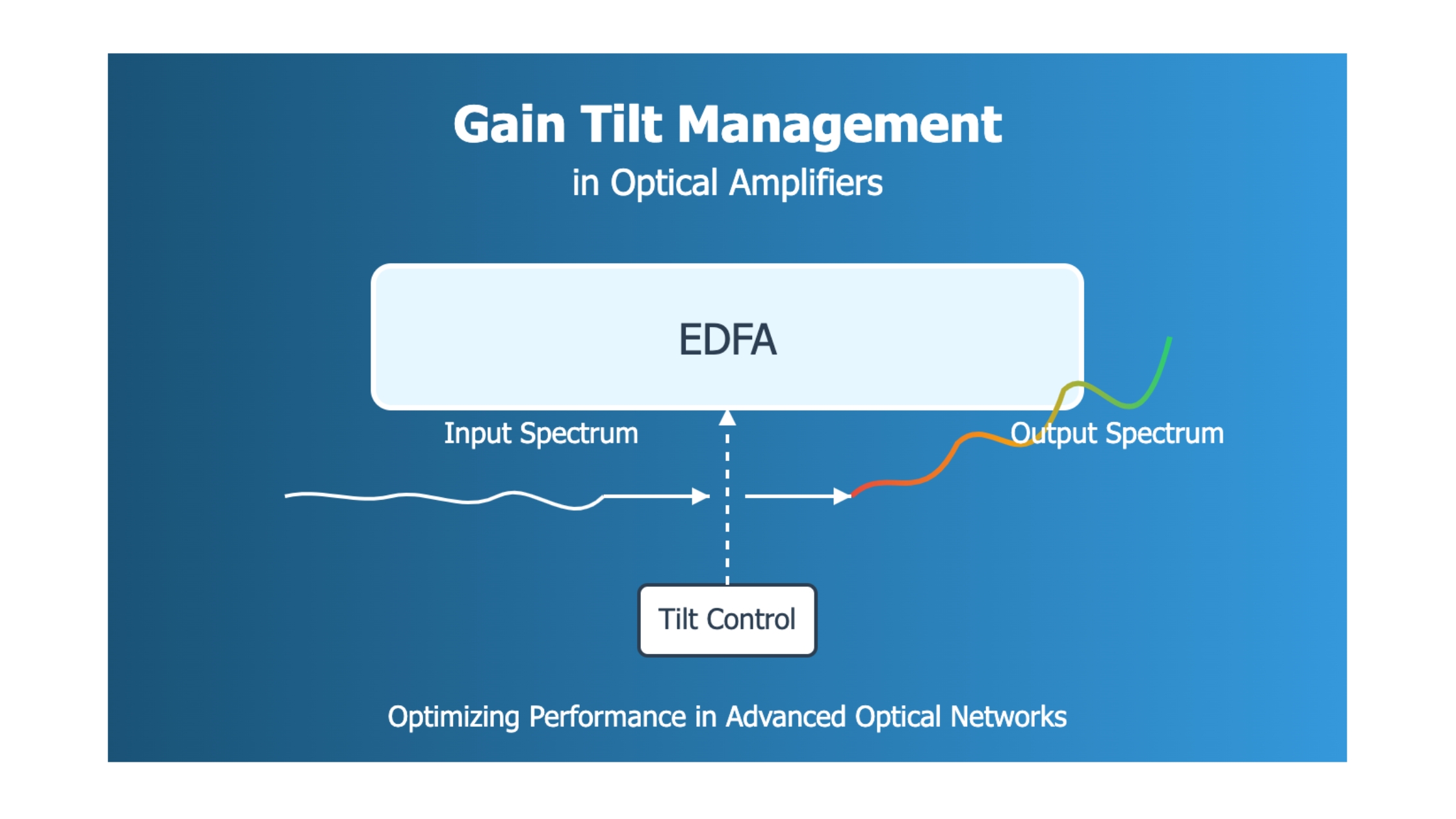
Where spectral slope comes from on an amplified DWDM line, how each contribution is quantified, and the order in which gain, tilt and per-slot corrections are applied.
- IEC 61291-4 parameters
- Inter-channel SRS 3.11 dB/span
- C+L 9.6 THz
- Tilt setpoint arithmetic
Pump power converts into gain, tilt and heat, in that order.
1. Introduction
A C-band erbium-doped fiber amplifier (EDFA) set to 20 dB of gain does not deliver 20 dB at every wavelength. The gain at 1530 nm and the gain at 1565 nm differ by an amount that changes whenever the amplifier is asked for a different gain, and the transmission fiber between amplifier sites adds a spectral slope of its own that scales with the total power launched into it. Neither effect averages out. Across a ten-span line both add span by span, and the channel at the depleted edge of the spectrum arrives with an optical signal-to-noise ratio (OSNR) several decibels below the channel at the other edge — which sets the reach of the whole system, because a line is engineered to its worst channel and not to its mean.
That systematic slope is gain tilt. It is not a defect to be eliminated but a quantity to be budgeted, commanded and monitored, in the same way span loss is. Every amplifier on a modern line accepts a tilt setpoint alongside its gain setpoint, and the number it is given comes from an arithmetic chain that starts at the fiber and ends at the control plane.
This article covers where each tilt contribution comes from, how each one is quantified from parameters a planning tool already holds, how the contributions accumulate along a cascade, and the order in which gain, tilt and per-slot corrections are applied. The boundary condition is a coherent line system with no inline dispersion compensation: the mid-stage of a two-stage amplifier now holds an attenuator and an equalizer rather than a dispersion-compensating module, which removes one historical tilt source and changes the arithmetic for the rest.
2. Gain Tilt Definition and Component Terms
Gain tilt is the systematic, close-to-linear variation of an optical amplifier's gain with wavelength across its operating band, quoted either as the gain difference between the two band edges in decibels or as a slope in dB/nm or dB/THz. Gain tilt captures the first-order slope only. The wavelength-fixed structure remaining around that slope is gain ripple, and the two are budgeted separately because only one of them can be commanded.
G(λ) = Pout(λ) − Pin(λ) [dB]
Tilt = G(λred) − G(λblue) [dB] · slope form: ∂G(λ)/∂λ [dB/nm]
Flatness = max G(λ) − min G(λ) [dB] · Ripple(λ) = G(λ) − fit(λ) [dB]
Where: G(λ) is the gain at wavelength λ, obtained from the output and input powers at that wavelength in dBm. λred and λblue are the long- and short-wavelength band edges, so the tilt is positive when the long-wavelength edge is favored. The slope form is the same quantity per unit wavelength and is what a fit reports. fit(λ) is the least-squares straight line through G(λ), so ripple is what survives after the tilt is removed. Typical ranges: C-band gain 20–30 dB, flatness specified at or below 1 dB across the band, tilt commanded in 0.1 dB steps.
Four neighbouring quantities get used interchangeably in operations, and each one answers a different question:
- Gain tilt against gain ripple. Tilt is the fitted slope and is commandable; ripple is the wavelength-fixed residual around that slope and is a property of the gain-flattening filter (GFF) and the erbium spectrum, so it repeats identically at every amplifier of the same type.
- Gain tilt against gain flatness. Flatness — multichannel gain variation in IEC 61291-4 terms — is the peak-to-peak spread of gain across the band and contains both tilt and ripple; a 1 dB flatness specification and a 1 dB tilt specification are different requirements on the same device.
- Amplifier gain tilt against line spectral tilt. Gain tilt is a property of the amplifier's transfer function; spectral tilt is the slope of the power profile arriving at a monitoring point, which is the sum of every amplifier's gain tilt and every span's transfer along the path.
- Multichannel gain tilt against operational tilt. IEC 61291-4 defines multichannel gain tilt as the ratio of the gain change in each channel to the gain change in a reference channel as the input conditions move from one set of channel powers to another — a sensitivity, dimensionless in the general case. The number an operator types into an amplifier is the simpler edge-to-edge gain difference at one operating point, in dB. Both are called tilt; only the second one has a setpoint.
Tilt [dB/nm] = ΔG [dB] ÷ Δλ [nm] · Tilt [dB/THz] = ΔG [dB] ÷ Δf [THz], with Δf = c·Δλ ÷ λ²
Where: ΔG is the edge-to-edge gain difference in dB (red edge minus blue edge, so a red-favored spectrum is positive); Δλ is the band width in nm; Δf is the same width in THz; c is the speed of light and λ the band centre wavelength. Typical ranges: an amplifier tilt setpoint spans roughly −5 to +5 dB across the C-band, commanded in 0.1 dB steps.
Practical Example — reading one gain sweep three ways
The spectrum in Figure 1 has a fitted gain of 22.00 dB at 1530 nm and 19.00 dB at 1565 nm, so its tilt is −3.00 dB across the band. Converting to a slope in wavelength gives −3.00 ÷ 35 = −0.086 dB/nm. Converting to frequency, 35 nm at 1550 nm is Δf = 3×10⁸ × 35×10⁻⁹ ÷ (1550×10⁻⁹)² = 4.37 THz, so the same tilt is −0.69 dB/THz. The measured curve peaks at 22.37 dB and bottoms at 18.62 dB, giving a flatness of 3.75 dB against a bound of |−3.00| + 1.20 = 4.20 dB. One sweep, three numbers, and only the first one is a setpoint.
Takeaway: Tilt is a single fitted number that an amplifier accepts as a command; ripple is a shape it cannot be told to remove. Every correction strategy in the rest of this article rests on that split — the tilt term is answered by amplifier setpoints, the ripple term only by a device with per-slot resolution.
3. Erbium Gain Shape and Gain-Dependent Tilt
Erbium in a silica host does not amplify uniformly. The emission and absorption cross-sections vary strongly with wavelength, and an unflattened C-band EDFA peaks near 1530 nm with 3 to 5 dB more gain there than in the 1560 nm region (measured, device literature). A gain-flattening filter removes that shape by inserting a matched wavelength-dependent loss, and the match is exact at exactly one operating point.
The reason a single filter cannot hold across the operating range is that erbium is homogeneously broadened. Changing the pump power changes the average population inversion, and changing the inversion changes the shape of the gain spectrum as well as its level. Raise the inversion and the 1530 nm peak grows faster than the 1560 nm shoulder; lower it and weight moves toward the red. A filter cut for one inversion therefore leaves a residual at any other, and the residual grows in proportion to how far the amplifier has moved from its design point.
This is why a line that measures flat at 17 dB of span loss can measure tilted at 24 dB, with nothing changed but the loss the amplifier is being asked to make up. It also explains an operational surprise that catches teams during capacity growth: adding channels raises the total input power, an amplifier in constant-gain mode raises its output to match, the inversion moves, and every downstream amplifier sees a spectrum whose slope has changed even though no setpoint was touched.
Takeaway: Gain-dependent tilt scales with the distance between the commanded gain and the gain the filter was cut for, so the cheapest tilt reduction available on any line is to operate amplifiers near their design gain — which is a span-loss and site-spacing decision made years before the first channel is lit.
4. Tilt Contributions Along an Amplified Span
Four terms decide the tilt correction at each amplifier site on a coherent line, and they do not share a sign. Two of them push power toward the red edge, one pushes toward the blue, and one depends on how the node was built. The tilt setpoint an amplifier is given is the negative of their sum, so getting the sum right matters more than getting any single term precisely right.
Wavelength-dependent span loss. Silica attenuation varies across the C-band, and published G.652.D fiber specifications hold the attenuation anywhere between 1525 nm and 1575 nm within 0.02 dB/km of its 1550 nm value (vendor-specified, fiber product datasheets). Over an 80 km span that bounds the C-band loss slope at 1.60 dB, with the blue edge attenuated more, which leaves the red edge higher. Extend the comb into the L-band and the term grows, because attenuation rises again beyond about 1600 nm.
Inter-channel stimulated Raman scattering (ISRS). Power transfers continuously from shorter wavelengths to longer ones inside the transmission fiber. The higher-frequency channels act as pumps and are depleted; the lower-frequency channels receive Raman gain. This term scales with the total power in the fiber and with the width of the occupied spectrum, which makes it the largest and the most load-dependent of the four. Section 5 quantifies it.
Amplifier gain-dependent tilt. The Section 3 mechanism, entering with the opposite sign when the amplifier runs above its filter design gain: higher inversion favors the blue edge, so this term partly cancels the two fiber terms rather than adding to them. That cancellation is accidental rather than designed, and it reverses on a short span where the amplifier runs below its design gain.
Node and filter shaping error. A wavelength-selective switch (WSS) has a port-to-port loss that varies mildly across the band, and every express path through a reconfigurable optical add-drop multiplexer (ROADM) adds one. The term is small per node and correlated across nodes of the same type, so a design allowance rather than a computed value is the normal treatment.
Sum the contributions with their signs before sizing the correction range. A design that budgets the largest single term and ignores the cancellation will specify more tilt range than the line needs on a long span, and too little on a short one where the amplifier term reverses.
4.1 Spectral Evolution From Launch to Correction
The same arithmetic looks different when it is drawn as a spectrum rather than a budget. A comb leaves the booster level, arrives at the next site with the accumulated slope on it, and leaves that site level again — and the small amount by which it fails to leave level is the whole subject of Section 6.
Takeaway: The correction at each site is the amplifier’s own gain-dependent shape plus one commanded number, and the command has a finite step size. Every span therefore contributes at least the quantization residual, before any error in the inputs is counted.
5. Inter-Channel SRS Tilt Model and Fiber Dependence
Raman power transfer between signal channels is the one tilt term that can be computed from parameters a planning tool already holds, and the computation is a single line. Over the width of a C-band or C+L comb the Raman gain profile of silica is close to linear in frequency separation, which reduces the coupled multi-channel problem to a closed-form expression for the transfer between the extreme channels.
ΔPISRS [dB] = 4.343 × Cr × Ptot × Leff × Δf
Where: ΔPISRS is the power transfer between the extreme channels of the comb in dB, positive toward the longer wavelength. Cr is the Raman gain slope of the fiber in 1/(W·km·THz), approximately 0.028 for a standard fiber of 80 µm² effective area, scaling inversely with effective area. Ptot is the total power launched into the span in W, converted from dBm before use. Leff = (1 − e−αL)/α is the effective length in km, with α the attenuation in 1/km, equal to α[dB/km] ÷ 4.343. Δf is the frequency separation between the extreme channels in THz — about 4.8 THz for a filled C-band and about 9.6 THz for a filled C+L. The constant 4.343 is 10/ln 10. Validity boundary: the linear approximation of the Raman profile holds to roughly 15 THz of comb width; beyond the gain peak near 13 THz the real profile turns over while the straight line keeps climbing, so the expression overstates transfer for wider combs.
Practical Example — inter-channel SRS tilt on the reference span
Take 80 km of G.652.D fiber at 0.20 dB/km. In linear units α = 0.20 ÷ 4.343 = 0.0461 /km, so Leff = (1 − e−3.684) ÷ 0.0461 = 21.17 km. A filled C-band comb at 21 dBm total launch is Ptot = 0.126 W across Δf = 4.8 THz, giving ΔPISRS = 4.343 × 0.028 × 0.126 × 21.17 × 4.8 = 1.56 dB — the value carried into the Figure 3 waterfall. Fill the L-band as well and Δf doubles to 9.6 THz, so the same total power produces 3.11 dB. Raise total launch from 21 dBm to 24 dBm and Ptot doubles in linear terms, so the transfer doubles again to 6.21 dB. Three decibels of extra launch power buys three decibels of extra tilt.
Two properties of that expression change how a line is operated rather than how it is designed. The transfer is proportional to the power present in the fiber, so a system provisioned for a full comb but running at 40% fill produces roughly 40% of the tilt, and a pre-tilt computed for full fill is wrong by decibels at the band edges. And the transfer is correlated span to span: every span of the same fiber carrying the same comb reproduces the same slope, so it accumulates linearly rather than averaging out. The practice of loading unused spectrum with shaped amplified spontaneous emission exists largely to hold the first of those properties constant from day one.
5.1 Fiber Dependence Through Effective Area
The Raman gain slope is a property of the fiber, not a constant of the model. Gain efficiency scales inversely with effective area, so a large-area fiber couples its channels more weakly, and the reduction outweighs the longer effective length that comes with lower attenuation. Holding Cr fixed while varying only attenuation gets the direction of the comparison wrong — it predicts that the fiber chosen for unrepeatered reach makes Raman transfer worse, when it makes it better. The detailed treatment of inter-band Raman transfer works this comparison through in full.
| Fiber class | Effective area (µm²) | Cr (1/W·km·THz) | Attenuation (dB/km) | Leff (km) | Inter-channel SRS tilt (dB) |
|---|---|---|---|---|---|
| G.652.D standard single-mode | 80 | 0.028 | 0.20 | 21.17 | 3.11 |
| G.655 non-zero dispersion shifted | 72 | 0.031 | 0.21 | 20.25 | 3.29 |
| G.654.E large effective area | 125 | 0.018 | 0.17 | 24.43 | 2.31 |
The G.654.E row carries about a quarter less tilt than the G.652.D row under identical launch conditions, despite a 15% longer effective length, because its effective area is more than half again as large. Effective-area values are the nominal figures for each class; the Cr entries for the 80 µm² and 72 µm² rows are the values used in the inter-channel SRS modeling literature, and the 125 µm² entry is scaled from them by effective area (computed).
Takeaway: Inter-channel SRS tilt is set by four numbers a planner already has — Raman gain slope, total launched power, effective length and comb width — and it is the only major tilt term that changes when a channel is added. Design the correction range against the fully loaded comb, then expect the working setpoint to track fill state rather than sit still.
6. Tilt Accumulation Across an Amplifier Cascade
A single span's tilt is a nuisance; eight spans of the same tilt is a system limit. Both the fiber terms and the amplifier term repeat with the same sign at every site of the same design, so they add span by span rather than averaging out — the defining property that separates tilt from a random impairment. Left uncorrected, the reference C+L span of Section 5 puts 3.11 dB into the spectrum each time, and an eight-span line arrives with roughly 25 dB between its edges, which no receiver dynamic range absorbs.
| Case | 1 span | 2 spans | 4 spans | 8 spans | 12 spans |
|---|---|---|---|---|---|
| Uncorrected (dB) | 3.11 | 6.22 | 12.44 | 24.88 | 37.32 |
| Residual, correlated (dB) | 0.30 | 0.60 | 1.20 | 2.40 | 3.60 |
| Residual, uncorrelated (dB) | 0.30 | 0.42 | 0.60 | 0.85 | 1.04 |
Deployed lines sit between the two residual laws. Part of the per-span error is systematic — a planning tool that under-estimates fill state, or a filter shape shared by every amplifier of the same model — and part is site-specific, coming from span-loss measurement error and connector variation. Treating the whole residual as uncorrelated is the optimistic assumption, and it is the one that produces a line that measures well at turn-up and drifts out of flatness three years later. The network-level strategy for spectral flatness sets the equalization interval from this arithmetic.
ΔOSNRedge = − Tiltend-to-end ÷ 2 [dB, relative to the band mean]
Where: ΔOSNRedge is the OSNR of the depleted band edge relative to the band average, and Tiltend-to-end is the accumulated tilt in dB at the receive terminal. The factor of two follows from the geometry: a linear tilt about a fixed band-average power puts each edge half the tilt away from the mean, and the amplified spontaneous emission floor is flat across the band to first order, so the power offset carries straight into OSNR. Worked example: eight spans at the correlated 0.30 dB residual give 2.40 dB end-to-end, so the depleted edge arrives 1.20 dB below the band average — 40% of a 3 dB system margin spent on flatness alone, before any impairment is counted.
Takeaway: Correction per span converts a linear accumulation into a residual accumulation, and the value of the correction is measured by which law that residual follows. A 0.30 dB residual is either a twelve-span problem or a non-problem, and only measurement across the cascade tells which.
7. Tilt Correction Elements and Their Ranges
Correction happens at four places on a line, and they answer different parts of the same spectrum. Two sit inside the amplifier, one sits in the node, and one sits at the transmitter. Choosing among them is a question of what shape needs removing: a first-order slope, a fixed ripple, or an arbitrary profile.
The gain loop is arithmetic on two scalars — total input power and total output power — and never resolves a channel. Wavelength dependence enters through the medium rather than the controller: because erbium is homogeneously broadened, the mid-stage attenuator setting selects one member of a one-parameter family of gain shapes, and that shape is applied optically to everything passing through at once. One commanded number therefore corrects a per-channel impairment, and it succeeds because inter-channel SRS transfer and loss slope are themselves indifferent to channel identity — each acts on a channel according to where it sits in the spectrum. The same fact bounds what the setpoint reaches: channel-to-channel differences pass through unchanged, the ripple is untouched, and a tilted full spectrum and a half-empty level one present the same total power to the same photodiode.
| Element | Spectral shape it corrects | Command granularity | What it costs |
|---|---|---|---|
| Amplifier tilt setpoint | First-order slope only | One number per amplifier, commanded in 0.1 dB steps | Mid-stage loss and a noise figure penalty; range is platform-dependent |
| Gain-flattening filter | The erbium shape at one design gain, ripple included | None — the profile is fixed when the filter is made | Fixed insertion loss and no adaptability once installed |
| Dynamic gain equalizer | Arbitrary profile: tilt, ripple and curvature | Loss per spectral bin, 6.25 GHz grid, with a slope limit per bin pair | Insertion loss in the mid-stage, module cost and control-plane work |
| Raman pump ratio | Broad slope across the band, set by pump wavelength mix | Relative power between pumps at different wavelengths | Pump power, optical safety procedure and gain-measurement time |
| Transmitter pre-emphasis | Predicted end-to-end slope, applied at the source | Per-channel launch power at the transponder | Launch-power headroom, and it goes stale when fill state changes |
The division of work is settled in current designs. Fixed shape belongs to the gain-flattening filter, first-order slope belongs to the amplifier setpoint, and everything left over belongs to a dynamic gain equalizer placed every few spans rather than at every site. Distributed Raman amplification adds a fifth option that changes the sign of the problem: because Raman gain is itself produced by power transfer toward longer wavelengths, a counter-propagating pump set placed correctly delivers gain and tilt correction in the same element, which is covered in the Raman amplification fundamentals guide.
Takeaway: Match the correction element to the shape, not to the site. An amplifier setpoint that is asked to remove ripple will trade one edge of the band for the other, and a dynamic gain equalizer installed where a setpoint would do buys insertion loss for a slope that was already commandable.
8. Amplifier Control Modes and Tilt Setpoint Derivation
An amplifier holds one of three things constant, and the choice changes what happens to tilt when the channel count moves. In constant-gain mode the controller adjusts pump power to keep output minus input fixed, so the spectral shape arriving at the input passes through unchanged and the inversion stays near its design point. In constant-output-power mode the controller holds total output fixed, so removing channels raises the power on the survivors, moves the inversion, and changes the gain shape — which is why a fiber cut on one degree can show up as a flatness alarm two nodes away. A third mode targets a per-channel power derived from the total output target and the channel count.
Pch [dBm] = Ptotal [dBm] − 10 · log10(Nch)
Where: Pch is the target power per channel in dBm at the amplifier output, Ptotal is the commanded total output power in dBm, and Nch is the number of channels the amplifier is carrying, counting shaped noise loading as channels where it is used. Worked example: a booster commanded to 20 dBm total across 96 channels targets 20 − 10·log10(96) = 20 − 19.82 = 0.18 dBm per channel. Fill only 48 of those channels without noise loading and the same total output puts 3.19 dBm on each — a 3 dB change in the nonlinear operating point that no tilt setpoint corrects.
Greq = Pgoal − Pavg · Gcmd = min( Gmax, max( Gmin, Greq ) )
Where: Pgoal is the per-channel output target in dBm from the expression above, Pavg is the measured average per-channel input power in dBm, and Gmin and Gmax bound the device gain range. A second constraint applies at the top end: if Pin + Greq would exceed the maximum total output power, the gain is limited to hold output at the ceiling. Both clamps raise an alarm, and both matter for tilt as well as for power — a clamped gain is by definition not the gain-flattening filter design gain, so the gain-dependent tilt term of Section 3 moves by TDGT times the amount the clamp took away.
The tilt setpoint itself is derived rather than measured, at least on first application. Each amplifier computes what the span ahead of it and the elements behind it will have done to the spectrum, and applies the negative of that sum:
Tset = −( Tacc + Tspan + Tnode ) + TDGT · ( G − Gdesign )
Where: Tset is the commanded tilt in dB, Tacc is the tilt accumulated upstream and carried to this node, Tspan is the sum of the inter-channel SRS and loss-slope terms computed for the span ahead, Tnode is the node shaping allowance, and the last term is the amplifier's own gain-dependent contribution from Section 3, which the controller cancels rather than adds. The residual after this arithmetic is what a dynamic gain equalizer is left to remove.
Tcmd = min( Tmax, max( Tmin, Tset ) ) · Tacc,out = Tset − Tcmd
Where: Tset is the derived setpoint, Tmin and Tmax bound the tilt range the device can apply, Tcmd is what it applies after clamping and quantization to the 0.1 dB step, and Tacc,out is the part it could not remove. That remainder is what the node publishes downstream as accumulated tilt, which is why a line whose amplifiers are running against their tilt limits shows a residual that grows site by site rather than staying flat.
Accumulated tilt travels between nodes on the optical supervisory channel alongside channel count, measured span loss and fiber type. Each amplifier reads the upstream state, adds what it expects its own span to contribute, sets gain and tilt, and publishes the updated state downstream. That chain is why fiber type has to be provisioned correctly at every site: an ILA told it is feeding G.652.D when the span is G.654.E will over-estimate the Raman term by roughly a quarter and command a tilt that is wrong in the same proportion, at every span, in the same direction.
Derived setpoints and measured correction answer different failure modes, and Section 9 works through both loops. The order in which they are applied at turn-up is set by the commissioning sequence for per-channel power.
Takeaway: Constant-gain mode preserves the spectrum through channel-count changes and constant-power mode does not, so the control mode chosen for an in-line amplifier is a tilt decision before it is a power decision.
9. Control Architecture and Parameter Exchange
No amplifier on a line computes its tilt setpoint from local information alone. The span ahead of it depends on fiber type and total launched power, and the spectrum arriving at it depends on what every upstream site did — so the setpoint is the output of a chain that runs the length of the line, carried between nodes on the optical supervisory channel (OSC) alongside the channel count, the measured span loss and the fiber type.
The relay is what makes a provisioning error expensive. A site told it is feeding G.652.D when the span is G.654.E over-estimates the Raman term by roughly a quarter, commands a tilt that is wrong by that proportion, and publishes an accumulated value that carries the error into every derivation below it. The error is systematic rather than random, so it accumulates under the linear law of Section 6 rather than the square-root one, and it is invisible at any single site.
Three layers separate the software that decides a setpoint from the hardware that executes it, and each runs at a different speed. Reading them as one system is what produces the common failure of a correct calculation applied too slowly to matter — or a fast loop chasing an objective nobody set.
The bottom layer is the reason a fiber cut does not take the surviving channels with it. When half the load disappears, the amplifier detects the input power drop and adjusts pump current before the surviving channels have moved far, with vendor-stated response in the sub-millisecond range. What it cannot do is decide whether the resulting spectrum is the one the line wants, because that judgement needs the span model and the published upstream state, both of which live a layer above.
9.1 Derived and Measured Correction
Two loops set the tilt on a working line, and they fail in opposite ways. A feed-forward loop predicts what the span will do and applies the answer before the spectrum arrives; it is instantaneous and needs no settling, and it is only as right as the fiber type, fill state and span loss it was given. A feedback loop reads the spectrum that arrived and corrects the difference; it is right whatever the inputs say, and it needs a settled line and a stable reference before it converges.
Apply the derived setpoints first and let the line settle, then close the measured loop against the arriving spectrum. Running the measured loop from the start makes it converge against a spectrum that is still moving, which either takes many iterations or settles on the wrong operating point.
Takeaway: A tilt setpoint is a control-plane output, not an amplifier property. It is derived from state published by the node upstream, executed by hardware two layers below the software that computed it, and corrected by a loop that only converges once the line has stopped moving.
10. Inter-Band Tilt in C+L Line Systems
Filling the L-band alongside the C-band roughly doubles the comb width and roughly doubles the aggregate power, and the inter-channel SRS expression of Section 5 is linear in both. In a fully loaded C+L system the inter-band transfer reaches approximately 8 dB per span, which is more than any amplifier tilt setpoint is designed to absorb on its own and more than the receiver dynamic range of the depleted band tolerates. That single number reshapes the architecture around it.
Band-dedicated amplification is the first consequence. Erbium in a standard host reaches usable gain across roughly 1530 to 1565 nm; reaching 1570 to 1610 nm requires a longer doped fiber at lower inversion, which produces a different gain shape and a higher noise figure — published amplifier specifications commonly place the L-band figure 0.5 to 2 dB above the C-band equivalent for the same gain (vendor-specified, platform-dependent). Every amplifier site therefore carries a C/L splitter at its input and a combiner at its output, two independent gain blocks, and two separately cut gain-flattening filters. The splitter pair consumes a guard band of typically 3 to 5 nm that no channel can occupy, and adds insertion loss to both bands. The design of C+L amplifier cascades works through the resulting budget.
The second consequence is that the residual stops being a straight line. Within each band the transfer is close to linear, but across the pair the profile that maximises the worst-channel generalized signal-to-noise ratio (GSNR) is curved rather than sloped, so a per-band tilt setpoint leaves a shape a setpoint cannot express. This is the clearest case where a dynamic gain equalizer earns its insertion loss: the correction needed is a profile, not a number.
The third consequence is operational. Because the transfer scales with total power in the fiber, every channel added to either band changes the operating point of every channel already in service. Lighting the first L-band carrier on a fiber carrying 96 C-band channels is not a small event — it moves the whole C-band spectrum, and the procedure for a hitless C to C+L migration exists to stage that change rather than take it in one step. Orchestrated turn-up, where channels are added in controlled groups with amplifier setpoints re-derived between groups, is the standard answer.
A pre-tilt computed for a fully loaded C+L comb is wrong by several decibels at the band edges when the line runs at 40% fill, because the Raman transfer scales with the power present. Either hold the fill state constant with shaped noise loading, or re-derive the setpoints whenever the occupied spectrum changes materially.
Takeaway: C+L operation converts tilt from an amplifier parameter into a system-level control loop. Two bands sharing one fiber are not two independent resources; they are one Raman-coupled medium whose spectral balance has to be commanded continuously.
11. Measurement, Acceptance and Operational Monitoring
Gain tilt is measured, not inferred, and the instrument matters. A laboratory characterisation sweeps a tunable source across the band and reads output power against input power at each wavelength, giving the full gain spectrum from which tilt, ripple and flatness are all extracted by fitting. In the field the equivalent measurement comes from an optical channel monitor at the amplifier input and output, which reports per-channel power on the live comb rather than a swept single tone — faster, continuous, and limited to the wavelengths that are lit.
CPV = max Pch − min Pch [dB] · Tilt error = Tmeasured − Tcommanded [dB]
Where: channel power variation (CPV) is the spread between the strongest and weakest channel at one measurement point, which is the line-level quantity a flatness budget is written against; the amplifier-level equivalents are the gain flatness and gain ripple of Section 2. Tilt error is the difference between what the fit reports and what the controller commanded, and it separates a device fault from a derivation fault: a device tracking its command correctly while the spectrum stays tilted means the derivation inputs are wrong, not the amplifier.
| Test | Configuration | What is read | Compared against |
|---|---|---|---|
| Gain spectrum sweep | Single tone stepped across the band at the specified input power and gain | Full gain against wavelength; tilt and ripple extracted by fitting | The flatness and tilt-accuracy figures on the amplifier specification |
| Tilt command accuracy | Commanded tilt stepped across its range at fixed gain | Fitted tilt of the measured spectrum at each step | Commanded value, step by step, including at both range ends |
| Gain-dependent tilt | Gain stepped across the operating range at fixed tilt command | Change in fitted tilt per dB of gain change | The dynamic gain tilt coefficient on the specification |
| Partial fill | Comb reduced to alternate channels, then to band edges only | Per-channel output power and the resulting spectral slope | The full-fill result, isolating load dependency from device behavior |
| Channel add and drop transient | A block of channels removed and restored while the survivors are monitored | Power excursion on surviving channels and time to settle | The transient specification, and the receiver's tolerance window |
| Cascade end-to-end | Full line at design fill, measured at every amplifier output | Tilt at each site, giving the per-span residual and its accumulation law | The flatness budget and the equalization interval derived from it |
The cascade measurement is the one that pays for itself. Measuring tilt at every amplifier output rather than only at the receive terminal separates the per-span residual from its accumulation, which is exactly the distinction Section 6 showed to be worth several spans of reach. A line whose residual grows linearly with site count has a systematic error to find — a fiber type provisioned wrongly, an amplifier model whose filter shape is common to every site, or a fill-state assumption that no longer holds. A line whose residual grows as the square root has ordinary site-to-site variation and needs no investigation.
In service, three quantities are worth trending rather than alarming on. The fitted tilt at each amplifier output shows whether setpoints are still valid as fill changes. The spread between the best and worst channel GSNR shows whether the tilt is costing margin or merely existing. And the difference between commanded and measured tilt shows an amplifier drifting toward the end of its range, which is a maintenance signal long before it is a fault. Reading those alongside the OSNR budget the line was designed to turns a flatness number into a margin statement.
Takeaway: A single end-of-line flatness measurement tells you that something is wrong. Measuring at every amplifier output tells you whether the cause is one site or every site, and that distinction decides whether the fix is a truck roll or a redesign.
12. Multi-Band Operation and Current Direction
Adding the S-band to a line takes the comb width past 15 THz, and the tilt problem changes character rather than scaling. A field-deployed transmission of 202.3 Tb/s over 15.6 THz of S+C+L bandwidth applied an experimentally optimized 5 dB pre-tilt across the occupied spectrum to answer the Raman transfer (measured, conference literature). Two things are notable in that number. It is smaller than the naive extrapolation of the Section 5 expression predicts, because past the Raman gain peak near 13 THz the real profile turns over while the linear approximation keeps climbing — the validity boundary stated in Section 5, reached in practice. And it was optimized experimentally rather than derived, which is the honest current state of wideband pre-tilt.
S-band amplification is the other constraint. Thulium-doped fiber amplifiers cover the band but use several pumps whose interaction with gain shape is nonlinear in the pump currents, so selecting a pump configuration that hits a target output power and a target gain shape at once is a numerical optimization rather than a lookup. Research effort has moved toward learned amplifier models that predict gain shape from input power profile and total power, and toward digital-twin control that computes power and tilt setpoints for the whole line against a GSNR objective rather than site by site. Both approaches replace a derived setpoint with a fitted one, and both need the measurement discipline of Section 11 to have any reference to fit against.
The direction of travel for terrestrial C+L systems in the meantime is steady rather than dramatic: per-slot equalization at more sites, shaped noise loading as the default rather than an option, and setpoint derivation moved from the amplifier into a controller that can see the whole path. None of that changes the physics in Sections 3 to 5. It changes who computes the number, and how often.
Takeaway: Wider bands make tilt correction a profile-fitting problem rather than a slope-setting one, and the linear inter-channel SRS expression that serves a C+L design well stops being trustworthy past about 15 THz of comb width. Check the model against the bandwidth before trusting its output.
13. Conclusion
Gain tilt sits at the junction of three things a network engineer already tracks separately: the physics of the gain medium, the nonlinear behavior of the fiber, and the control plane that ties amplifiers into a line. Treating it as an amplifier property alone leads to correction ranges sized against the wrong term and setpoints that go stale as the spectrum fills. Treating it as a budget — four contributions with signs, accumulating across a cascade under a law that measurement can identify — turns it into an ordinary engineering quantity with a worked answer at every stage.
The mechanisms are settled and the arithmetic is short. What is still moving is the width of the spectrum being managed and the level at which the setpoints are computed, and both are moving in the same direction: wider bands, more coupling between channels that were once independent, and control that reaches across the whole path rather than one site at a time. An engineer who can compute the four contributions for a span and name which of them changes when a channel is added is ready for that shift, because the terms do not change when the band count does. Only their size does.
References
- ITU-T Recommendation G.661 — Definitions and test methods for the relevant generic parameters of optical amplifier devices and subsystems, ITU-T Study Group 15.
- ITU-T Recommendation G.662 — Generic characteristics of optical amplifier devices and subsystems, ITU-T Study Group 15.
- ITU-T Recommendation G.665 — Generic characteristics of Raman amplifiers and Raman amplified subsystems, ITU-T Study Group 15.
- IEC 61291-4 — Optical amplifiers, Part 4: Multichannel applications, International Electrotechnical Commission.
- ITU-T G-series Supplement 39 — Optical system design and engineering considerations, ITU-T Study Group 15.
- ITU-T Recommendation G.652 — Characteristics of a single-mode optical fiber and cable, ITU-T Study Group 15.
- ITU-T Recommendation G.694.1 — Spectral grids for WDM applications: DWDM frequency grid, ITU-T Study Group 15.
Related Articles on MapYourTech