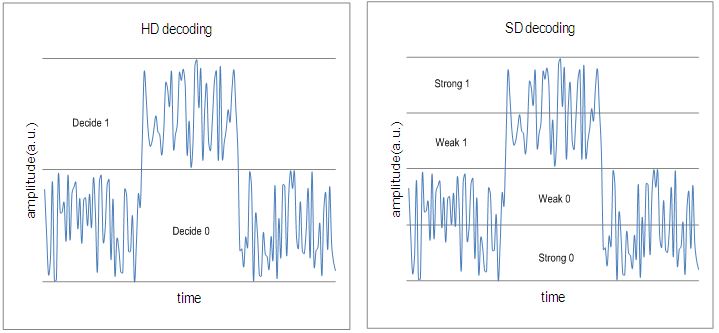
MapYourTech Complete Banner - Scoped CSS
Tag

Signal quality

Browsing
Fundamentals of Noise Figure in Optical Amplifiers

Noise figure (NF) is a critical parameter in optical amplifiers that quantifies the degradation of signal-to-noise ratio during amplification. In multi-span optical networks, the accumulated noise from cascaded amplifiers ultimately determines system reach, capacity, and performance.

While amplifiers provide the necessary gain to overcome fiber losses, they inevitably add amplified spontaneous emission (ASE) noise to the signal. The noise contribution from each amplifier accumulates along the transmission path, with early-stage amplifiers having the most significant impact on the end-to-end system performance.

Understanding the noise behavior in cascaded amplifier chains is fundamental to optical network design. This article explores noise figure fundamentals, calculation methods, and the cumulative effects in multi-span networks, providing practical design guidelines for optimizing system performance.

Definition and Physical Meaning

Noise figure is defined as the ratio of the input signal-to-noise ratio (SNR) to the output SNR of an amplifier, expressed in decibels (dB):

NF = 10 log₁₀(SNRin / SNRout) dB

Alternatively, it can be expressed using the noise factor F (linear scale):

NF = 10 log₁₀(F) dB

In optical amplifiers, the primary noise source is amplified spontaneous emission (ASE), which originates from spontaneous transitions in the excited gain medium. Instead of being stimulated by the input signal, these transitions occur randomly and produce photons with random phase and direction.

Noise Figure Fundamentals Optical Amplifier Clean signal SNRin Signal + ASE noise SNRout ASE generation NF = 10 log₁₀(SNRin / SNRout) dB = 10 log₁₀(1 + PASE/(G·Psignal)) dB

Quantum Limit and Physical Interpretation

Even a theoretically perfect amplifier has a quantum-limited minimum noise figure of 3dB. This fundamental limit exists because the amplification process inherently introduces at least half a photon of noise per mode.

The noise figure is related to several physical parameters:

  • Spontaneous Emission Factor (nsp): Represents the quality of population inversion in the active medium
  • Population Inversion: The ratio of atoms in excited states versus ground states
  • Quantum Efficiency: How efficiently pump power creates population inversion
NF = 2·nsp·(1-1/G)

As gain (G) becomes large, this approaches: NF = 2·nsp, with a theoretical minimum of 3dB when nsp = 1.

Factors Affecting Noise Figure

Gain and Population Inversion

The population inversion level directly affects the noise figure. Higher inversion leads to lower ASE and therefore lower noise figure. Key relationships include:

  • Gain Level: Higher gain typically results in better inversion and lower NF up to a saturation point
  • Pump Power: Increased pump power improves inversion up to a saturation level
  • Gain Medium Length: Longer gain medium increases available gain but can increase NF if inversion is not maintained throughout

Input Power Dependence

Noise figure varies with input signal power:

  • At very low input powers, the gain can be higher but the effective NF may increase due to insufficient saturation
  • At high input powers, gain saturation occurs, leading to a higher effective NF
  • The optimal input power range for lowest NF is typically 10-15dB below the saturation input power
Noise Figure vs. Input Power Input Power (dBm) -30 -20 -10 0 +10 Noise Figure (dB) 4 5 6 7 8 9 High NF region (Low input power) Optimal operating region High NF region (Gain saturation)

Wavelength Dependence

Noise figure typically varies across the operating wavelength band:

  • The wavelength dependence follows the gain spectrum of the amplifier
  • In typical optical amplifiers, NF is often lowest near the peak gain wavelength
  • Edge wavelengths generally experience higher NF due to lower inversion and gain
  • This wavelength dependence can impact system design, especially for wideband applications

Temperature Effects

Temperature significantly impacts noise figure performance:

  • Higher temperatures typically increase NF due to reduced population inversion efficiency
  • Temperature-dependent cross-sections in the gain medium affect both gain and noise performance
  • Thermal management is critical for maintaining consistent NF performance, especially in high-power amplifiers

EDFA Specifications

In optical networks, various EDFA designs are available with specific noise figure performance characteristics:

Application Typical NF Range Typical Gain Range
Metro access 6.0-7.0dB 12-21dB
Metro/regional 5.5-6.5dB 14-22dB
Regional with mid-stage access 5.5-7.5dB 15-28dB
Long-haul with mid-stage access 5.0-7.0dB 25-37dB
Regional single-stage 5.0-6.0dB 15-28dB
Long-haul single-stage 5.0-6.0dB 25-37dB
Ultra-short span booster 15.0-17.0dB 5-7dB

Temperature Sensitivity

Noise figure is temperature sensitive, with performance typically degrading at higher temperatures due to:

  • Reduced pump efficiency
  • Changes in population inversion
  • Increased thermal noise contributions

Most optical amplifiers are designed to operate in accordance with standard telecom environmental specifications like ETS 300 019-1-3 Class 3.1E for environmental endurance.

Cascaded Amplifiers and Noise Accumulation

In optical networks, signals typically pass through multiple amplifiers as they traverse through fiber spans. Understanding how noise accumulates in these multi-span systems is critical for designing networks that meet performance requirements.

Friis' Formula and Cascaded Amplifier Systems

The noise accumulation in a chain of optical amplifiers follows Friis' formula, which was originally developed for electronic amplifiers but applies equally to optical systems:

Ftotal = F1 + (F2-1)/G1 + (F3-1)/(G1·G2) + ... + (Fn-1)/(G1·G2···Gn-1)

Where:

  • Ftotal is the total noise factor (linear, not in dB)
  • Fi is the noise factor of the i-th amplifier
  • Gi is the gain (linear) of the i-th amplifier

In optical systems, this formula must account for span losses between amplifiers:

Ftotal = F1 + (L1·F2-1)/G1 + (L1·L2·F3-1)/(G1·G2) + ...

Where Li represents the span loss (linear) between amplifiers i and i+1.

Cascaded Amplifier System Amp 1 NF₁ = 5dB Span 1 Loss = 20dB Amp 2 NF₂ = 5dB Span 2 Loss = 20dB Amp 3 NF₃ = 5dB Span N Amp N NFₙ = 5dB Accumulated Noise OSNR final ≈ P launch − L span − NF − 10log 10 (N) − 58

Key Insights from Friis' Formula

The most significant insight from Friis' formula is that the first amplifier has the most substantial impact on the overall noise performance. Each subsequent amplifier's noise contribution is reduced by the gain of all preceding amplifiers.

Practical implications include:

  • Always use the lowest noise figure amplifier at the beginning of a chain
  • The impact of noise figure improvements diminishes for amplifiers later in the chain
  • Pre-amplifiers are more critical for noise performance than boosters
  • Mid-stage components (like DCFs) should have minimal loss to preserve good noise performance

OSNR Evolution in Multi-span Systems

The optical signal-to-noise ratio (OSNR) evolution through a multi-span system can be approximated by:

OSNRdB ≈ Plaunch - α·L - NF - 10·log10(N) - 10·log10(Bref) + 58

Where:

  • Plaunch is the launch power per channel (dBm)
  • α is the fiber attenuation coefficient (dB/km)
  • L is the span length (km)
  • NF is the amplifier noise figure (dB)
  • N is the number of spans
  • Bref is the reference bandwidth for OSNR measurement (typically 0.1nm)
  • 58 is a constant that accounts for physical constants (h𝜈)

The key insight from this equation is that OSNR degrades by 3dB each time the number of spans doubles (10·log10(N) term). This creates a fundamental limit to transmission distance in amplified systems.

Practical Example: OSNR Calculation in a Multi-span System

Consider a 10-span system with the following parameters:

  • Launch power: +1dBm per channel
  • Span length: 80km
  • Fiber loss: 0.2dB/km (total span loss = 16dB)
  • Amplifier gain: 16dB (exactly compensating span loss)
  • Amplifier noise figure: 5dB
  • Reference bandwidth: 0.1nm (~12.5GHz at 1550nm)

Step 1: Calculate the OSNR for a single span:

OSNR1-span = +1 - 16 - 5 - 10·log10(1) - 10·log10(12.5) + 58
= +1 - 16 - 5 - 0 - 11 + 58 = 27dB

Step 2: Calculate the OSNR degradation due to multiple spans:

OSNR degradation = 10·log10(N) = 10·log10(10) = 10dB

Step 3: Calculate the final OSNR:

OSNR10-spans = OSNR1-span - 10·log10(N) = 27 - 10 = 17dB

With a typical OSNR requirement of 12-15dB for modern coherent transmission formats, this system has adequate margin for reliable operation. However, extending to 20 spans would reduce OSNR by another 3dB to 14dB, approaching the limit for reliable operation.

Multi-Stage Amplifier Design

Based on the principles of Friis' formula, multi-stage amplifiers with optimal noise performance typically follow a design where:

Multi-Stage Amplifier Design Optimal Design Low NF Pre-Amp Power Amp Component NF = 4.5dB G = 15dB Loss = 1dB NF = 6.5dB G = 15dB Impact if First Stage NF = 6.5dB: Overall NF increases by ~2dB Impact if Second Stage NF = 8.5dB: Overall NF increases by only ~0.2dB

Key design principles include:

  • Low-Noise First Stage: The first stage should be optimized for low noise figure, even at the expense of output power capability
  • Power-Optimized Second Stage: The second stage can focus on power handling and efficiency once the SNR has been established by the first stage
  • Minimal Mid-Stage Loss: Any passive components (filters, isolators, etc.) between stages should have minimal insertion loss to avoid degrading the noise performance

EDFA Models and Cascaded Performance

Various types of optical amplifiers are designed with cascaded performance in mind:

Type Mid-Stage Features Design Optimization
Variable gain with mid-stage access Mid-stage access for DCF Optimized for regional networks
High-gain variable gain with mid-stage access Mid-stage access for DCF Optimized for high-gain applications
Variable gain with mid-stage access
and C/T filters
Mid-stage access for DCF Optimized for high-power applications
with OSC handling

Typical mid-stage dispersion compensation fiber (DCF) parameters tracked in optical networks include dispersion value, PMD, and tilt, which are critical for maintaining overall system performance.

Automatic Laser Shutdown (ALS) and Safety

In high-power multi-span systems, safety mechanisms like Automatic Laser Shutdown (ALS) are implemented to prevent hazardous conditions during fiber breaks or disconnections:

  • ALS triggers when LOS (Loss Of Signal) is detected on a line port
  • During ALS, EDFAs are disabled except for periodic 30-second probing intervals at reduced power (20dBm)
  • Normal operation resumes only after signal restoration for at least 40 seconds

Modern optical amplifiers feature ALS functionality with configurable parameters to ensure both optimal performance and safety in cascaded environments.

Network Applications and Optimization Strategies for Optical Amplifiers

Different segments of optical networks have varying requirements for noise figure performance based on their application, reach requirements, and economic considerations.

Network Segment Requirements

Noise Figure Requirements by Network Segment Access Short reach High splitting loss Metro/Regional Medium reach Mixed node types Long-haul Extended reach Many cascaded amps Typical NF Req: 6-7 dB (Less critical) Typical NF Req: 5-6 dB (Balanced design) Typical NF Req: 4-5 dB (Highly critical) Design Focus: • Cost efficiency • Size/integration Design Focus: • Flexibility • Dynamic range Design Focus: • Minimal NF • Optimized cascade

Access Networks

Access networks are generally tolerant of higher noise figures (6-7dB) because:

  • They involve fewer amplifiers in cascade
  • They often operate with higher channel powers
  • Transmission distances are relatively short
  • Cost sensitivity is higher than performance optimization

Metro/Regional Networks

Metro and regional networks require balanced NF performance (5-6dB) with:

  • Good dynamic range to handle varying traffic patterns
  • Flexibility to support different node configurations
  • Moderate reach capabilities (typically 4-10 spans)
  • Reasonable cost-performance trade-offs

Long-haul Networks

Long-haul and submarine networks demand optimized low-NF designs (4-5dB) due to:

  • Large number of amplifiers in cascade (often 10-20+)
  • Need to maximize reach without electrical regeneration
  • Requirement to support advanced modulation formats
  • Justification for premium components due to overall system economics

Economic Implications of Noise Figure

Improving noise figure comes with cost implications that must be carefully evaluated:

NF Improvement Typical Cost Increase Performance Benefit Economic Justification
6.0dB → 5.5dB +5-10% ~10% reach increase Generally cost-effective
5.5dB → 5.0dB +10-15% ~10% reach increase Often justified for long-haul
5.0dB → 4.5dB +15-25% ~10% reach increase Specialty applications only
4.5dB → 4.0dB +30-50% ~10% reach increase Rarely justified economically

The economic tradeoffs include:

  • Capital vs. Operating Expenses: Higher-quality, lower-NF amplifiers cost more initially but may reduce the need for additional amplifier sites and regeneration points
  • Upgrade Paths: Better NF provides margin for future capacity upgrades with more advanced modulation formats
  • Lifecycle Considerations: Premium amplifiers may maintain better performance over their operational lifetime, delaying replacement needs
  • System Capacity: Improved NF can enable higher capacity through better OSNR margin, often at lower cost than adding new fiber routes

Operational Optimization Strategies

For system operators using EDFAs, several practical optimization strategies can help maximize performance:

1. Gain Optimization

Modern optical amplifiers support different operation modes with specific gain management approaches:

  • Automatic Mode: Maintains output power per channel based on saturation power and maximum channel count settings
  • Semi-automatic Mode: Maintains a fixed output power per channel
  • Constant Gain Mode: Maintains a fixed gain regardless of input power variations
  • Automatic Power Control (APC) Mode: Provides automatic power control for specialized applications
  • Automatic Current Control (ACC) Mode: Provides precise pump current control for specialized applications

Advanced amplifiers implement specific algorithms for gain control that include careful monitoring of required gain versus actual gain, with alarms for out-of-range or out-of-margin conditions.

2. Tilt Management

Spectral tilt management is crucial for maintaining consistent OSNR across all channels:

  • Modern EDFAs automatically adjust tilt to compensate for fiber and component tilt
  • SRS (Stimulated Raman Scattering) tilt compensation is included for high-power systems
  • Built-in tilt values are stored in amplifier memory and used as reference points
  • For ultra-short span boosters and extended C-band amplifiers, specialized tilt algorithms account for fiber type

3. Temperature Control

Optical amplifiers typically specify operational temperature ranges in accordance with telecom standards like ETS 300 019-1-3 Class 3.1E, emphasizing the importance of controlling environmental conditions to maintain optimal performance.

4. Fiber Plant Optimization

Several fiber plant parameters impact noise figure performance:

  • Span Loss: Monitored and alarmed when outside expected range
  • Mid-stage Loss: For dual-stage amplifiers, carefully managed for optimal performance
  • Transmission Fiber Type: Configuration option that affects SRS tilt compensation
  • DCF Parameters: Dispersion, PMD, and tilt tracked in network control protocols

Noise Figure Design Guidelines

  1. Place Highest Quality First: Always use the lowest noise figure amplifiers at the beginning of the chain where they have the most impact
  2. Budget Wisely: Budget 0.5-1.0dB extra margin for each amplifier to account for aging and temperature variations over the system lifetime
  3. Consider Total Cost: Evaluate the total cost impact of NF improvements, including reduced regeneration needs and extended reach capabilities
  4. Monitor Trends: Establish baseline NF measurements and monitor for gradual degradation that might indicate pump laser aging
  5. Balance Requirements: Balance NF with other parameters like output power, gain flatness, and dynamic range based on specific application needs
  6. Test Under Load: Validate NF performance under realistic channel loading conditions, not just with a single test wavelength

Future Trends in Noise Figure Technology

Future Trends in Noise Figure Technology AI-Optimized Amplifiers Machine Learning Parameter Optimization Advanced Materials Novel Dopants & Co-dopants Engineered Glass Structures Integrated Photonics On-Chip Amplification Hybrid Integration Quantum Approaches Quantum-Enhanced Amplification Phase-Sensitive Designs

Emerging technologies for noise figure optimization include:

  • AI-Driven Optimization: Machine learning algorithms that dynamically adjust amplifier parameters based on real-time network conditions
  • Advanced Material Science: New dopant materials and glass compositions that enable better population inversion and reduced spontaneous emission
  • Integrated Photonics: Silicon photonics and other integrated platforms that combine amplification with filtering and control functions
  • Quantum-Enhanced Amplification: Phase-sensitive amplification and other quantum approaches that can theoretically break the 3dB quantum noise limit
  • Distributed Intelligence: Network-wide optimization that coordinates multiple amplifiers for global noise minimization

EDFA Implementation Examples

Metro Network Design

A typical metro network implementation might include:

  • Terminal nodes using fixed-gain boosters and pre-amplifiers
  • FOADM nodes using low-gain pre-amplifiers
  • Flexible OADM nodes employing medium-gain boosters

Regional Network Design

For regional networks, typical designs include:

  • Terminal nodes with AWG Mux/DeMux and EDFAs for amplification
  • Modern terminals with WSS for automatic equalization
  • ROADM nodes employing pre-amplifiers with mid-stage access for DCF compensation and boosters
  • In-line amplifier nodes (ILAN) using EDFAs to compensate for transmission fiber and DCF loss

Specialized Applications

Some specialized EDFA designs address unique requirements:

  • Ultra-short span boosters: Very high output power (26dBm) with narrow gain range (5-7dB)
  • High-power pre-amps: For ROADM applications with specialized eye-safety verification process
  • Pluggable EDFAs: For applications requiring compact, modular amplification in form factors like CFP2

Conclusion

Noise figure is a fundamental parameter that sets ultimate performance limits for optical amplifier systems. Modern EDFA families demonstrate a comprehensive approach to addressing various network requirements with optimized designs for different applications.

Key takeaways include:

  • Noise figure quantifies an amplifier's SNR degradation, with a quantum-limited minimum of 3dB
  • In cascaded configurations, noise accumulates according to Friis' formula, with early-stage amplifiers having the most significant impact
  • Network operators can optimize NF through proper pump power settings, gain optimization, temperature control, and careful wavelength planning
  • Multi-stage designs with low-NF first stages offer the best overall performance for critical applications
  • Economic considerations must balance the additional cost of lower-NF amplifiers against improved system reach and capacity

The evolution of EDFA technology reflects the ongoing refinement of noise figure optimization techniques, with newer designs and features continually addressing the evolving requirements of optical networks.

Optical networks are the backbone of the internet, carrying vast amounts of data over great distances at the speed of light. However, maintaining signal quality over long fiber runs is a challenge due to a phenomenon known as noise concatenation. Let’s delve into how amplified spontaneous emission (ASE) noise affects Optical Signal-to-Noise Ratio (OSNR) and the performance of optical amplifier chains.

The Challenge of ASE Noise

ASE noise is an inherent byproduct of optical amplification, generated by the spontaneous emission of photons within an optical amplifier. As an optical signal traverses through a chain of amplifiers, ASE noise accumulates, degrading the OSNR with each subsequent amplifier in the chain. This degradation is a crucial consideration in designing long-haul optical transmission systems.

Understanding OSNR

OSNR measures the ratio of signal power to ASE noise power and is a critical parameter for assessing the performance of optical amplifiers. A high OSNR indicates a clean signal with low noise levels, which is vital for ensuring data integrity.

Reference System for OSNR Estimation

As depicted in Figure below), a typical multichannel N span system includes a booster amplifier, N−1 line amplifiers, and a preamplifier. To simplify the estimation of OSNR at the receiver’s input, we make a few assumptions:

Representation of optical line system interfaces (a multichannel N-span system)
  • All optical amplifiers, including the booster and preamplifier, have the same noise figure.
  • The losses of all spans are equal, and thus, the gain of the line amplifiers compensates exactly for the loss.
  • The output powers of the booster and line amplifiers are identical.

Estimating OSNR in a Cascaded System

E1: Master Equation For OSNR

E1: Master Equation For OSNR

Pout is the output power (per channel) of the booster and line amplifiers in dBm, L is the span loss in dB (which is assumed to be equal to the gain of the line amplifiers), GBA is the gain of the optical booster amplifier in dB, NFis the signal-spontaneous noise figure of the optical amplifier in dB, h is Planck’s constant (in mJ·s to be consistent with Pout in dBm), ν is the optical frequency in Hz, νr is the reference bandwidth in Hz (corresponding to c/Br ), N–1 is the total number of line amplifiers.

The OSNR at the receivers can be approximated by considering the output power of the amplifiers, the span loss, the gain of the optical booster amplifier, and the noise figure of the amplifiers. Using constants such as Planck’s constant and the optical frequency, we can derive an equation that sums the ASE noise contributions from all N+1 amplifiers in the chain.

Simplifying the Equation

Under certain conditions, the OSNR equation can be simplified. If the booster amplifier’s gain is similar to that of the line amplifiers, or if the span loss greatly exceeds the booster gain, the equation can be modified to reflect these scenarios. These simplifications help network designers estimate OSNR without complex calculations.

1)          If the gain of the booster amplifier is approximately the same as that of the line amplifiers, i.e., GBA » L, above Equation E1 can be simplified to:

osnr_2

E1-1

2)          The ASE noise from the booster amplifier can be ignored only if the span loss L (resp. the gain of the line amplifier) is much greater than the booster gain GBA. In this case Equation E1-1 can be simplified to:

E1-2

3)          Equation E1-1 is also valid in the case of a single span with only a booster amplifier, e.g., short‑haul multichannel IrDI in Figure 5-5 of [ITU-T G.959.1], in which case it can be modified to:

E1-3

4)          In case of a single span with only a preamplifier, Equation E1 can be modified to:

Practical Implications for Network Design

Understanding the accumulation of ASE noise and its impact on OSNR is crucial for designing reliable optical networks. It informs decisions on amplifier placement, the necessity of signal regeneration, and the overall system architecture. For instance, in a system where the span loss is significantly high, the impact of the booster amplifier on ASE noise may be negligible, allowing for a different design approach.

Conclusion

Noise concatenation is a critical factor in the design and operation of optical networks. By accurately estimating and managing OSNR, network operators can ensure signal quality, minimize error rates, and extend the reach of their optical networks.

In a landscape where data demands are ever-increasing, mastering the intricacies of noise concatenation and OSNR is essential for anyone involved in the design and deployment of optical communication systems.

References

https://www.itu.int/rec/T-REC-G/e

Items HD-FEC SD-FEC
Definition Decoding based on hard-bits(the output is quantized only to two levels) is called the “HD(hard-decision) decoding”, where each bit is considered definitely one or zero. Decoding based on soft-bits(the output is quantized to more than two levels) is called the “SD(soft-decision) decoding”, where not only one or zero decision but also confidence information for the decision are provided.
Application Generally for non-coherent detection optical systems, e.g.,  10 Gbit/s, 40 Gbit/s, also for some coherent detection optical systems with higher OSNR coherent detection optical systems, e.g.,  100 Gbit/s,400 Gbit/s.
Electronics Requirement ADC(Analogue-to-Digital Converter) is not necessary in the receiver. ADC is required in the receiver to provide soft information, e.g.,  coherent detection optical systems.
specification general FEC per [ITU-T G.975];super FEC per [ITU-T G.975.1]. vendor specific
typical scheme Concatenated RS/BCH LDPC(Low density parity check),TPC(Turbo product code)
complexity medium high
redundancy ratio generally 7% around 20%
NCG about 5.6 dB for general FEC;>8.0 dB for super FEC. >10.0 dB
 Example(If you asked your friend about traffic jam status on roads and he replies) maybe fully jammed or free  50-50  but I found othe way free or less traffic

Optical power tolerance: It refers to the tolerable limit of input optical power, which is the range from sensitivity to overload point.

Optical power requirement: If refers to the requirement on input optical power, realized by adjusting the system (such as adjustable attenuator, fix attenuator, optical amplifier).


Optical power margin: It refers to an acceptable extra range of optical power. For example, “–5/ + 3 dB” requirement is actually a margin requirement.

When the bit error occurs to the system, generally the OSNR at the transmit end is well and the fault is well hidden.
Decrease the optical power at the transmit end at that time. If the number of bit errors decreases at the transmit end, the problem is non-linear problem.
If the number of bit errors increases at the transmit end, the problem is the OSNR degrade problem. 


General Causes of Bit Errors

  •  Performance degrade of key boards
  • Abnormal optical power
  • Signal-to-noise ratio decrease
  • Non-linear factor
  • Dispersion (chromatic dispersion/PMD) factor
  • Optical reflection
  • External factors (fiber, fiber jumper, power supply, environment and others)

The main advantages and drawbacks of EDFAs are as follows.

Advantages

  • Commercially available in C band (1,530 to 1,565 nm) and L band (1,560 to 1,605) and up to  84-nm range at the laboratory stage.
  • Excellent coupling: The amplifier medium is an SM fiber;
  • Insensitivity to light polarization state;
  • Low sensitivity to temperature;
  • High gain: > 30 dB with gain flatness < ±0.8 dB and < ±0.5 dB in C and L band, respectively, in the scientific literature and in the manufacturer documentation
  • Low noise figure: 4.5 to 6 dB
  • No distortion at high bit rates;
  • Simultaneous amplification of wavelength division multiplexed signals;
  • Immunity to crosstalk among wavelength multiplexed channels (to a large extent)

Drawbacks

  • Pump laser necessary;
  • Difficult to integrate with other components;
  • Need to use a gain equalizer for multistage amplification;
  • Dropping channels can give rise to errors in surviving channels:dynamic control of amplifiers is  necessary.

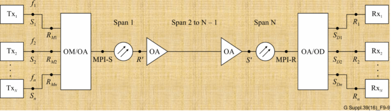
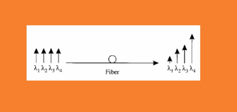
In a non-coherent WDM system, each optical channel on the line side uses only one binary channel to carry service information. The service transmission rate on each optical channel is called bit rate while the binary channel rate is called baud rateIn this sense, the baud rate was equal to the bit rate. The spectral width of an optical signal is determined by the baud rate. Specifically, the spectral width is linearly proportional to the baud rate, which means a higher baud rate generates a larger spectral width.

  • Baud (pronounced as /bɔ:d/ and abbreviated as “Bd”) is the unit for representing the data communication speed. It indicates the signal changes occurring in every second on a device, for example, a modulator-demodulator (modem). During encoding, one baud (namely, the signal change) actually represents two or more bits. In the current high-speed modulation techniques, each change in a carrier can transmit multiple bits, which makes the baud rate different from the transmission speed.

In practice, the spectral width of the optical signal cannot be larger than the frequency spacing between WDM channels; otherwise, the optical spectrums of the neighboring WDM channels will overlap, causing interference among data streams on different WDM channels and thus generating bit errors and a system penalty.

For example, the spectral width of a 100G BPSK/DPSK signal is about 50 GHz, which means a common 40G BPSK/DPSK modulator is not suitable for a 50 GHz channel spaced 100G system because it will cause a high crosstalk penalty. When the baud rate reaches 100 Gbaud/s, the spectral width of the BPSK/DPSK signal is greater than 50 GHz. Thus, it is impossible to achieve 50 GHz channel spacing in a 100G BPSK/DPSK transmission system.

(This is one reason that BPSK cannot be used in a 100G coherent system. The other reason is that high-speed ADC devices are costly.)

A 100G coherent system must employ new technology. The system must employ more advanced multiplexing technologies so that an optical channel contains multiple binary channels. This reduces the baud rate while keeping the line bit rate unchanged, ensuring that the spectral width is less than 50 GHz even after the line rate is increased to 100 Gbit/s. These multiplexing technologies include quadrature phase shift keying (QPSK) modulation and polarization division multiplexing (PDM).

For coherent signals with wide optical spectrum, the traditional scanning method using an OSA or inband polarization method (EXFO) cannot correctly measure system OSNR. Therefore, use the integral method to measure OSNR of coherent signals.

Perform the following operations to measure OSNR using the integral method:

1.Position the central frequency of the wavelength under test in the middle of the screen of an OSA.
2.Select an appropriate bandwidth span for integration (for 40G/100G coherent signals, select 0.4 nm).
3.Read the sum of signal power and noise power within the specified bandwidth. On the OSA, enable the Trace Integ function and read the integral value. As shown in Figure 2, the integral optical      power (P + N) is 9.68 uW.
4.Read the integral noise power within the specified bandwidth. Disable the related laser before testing the integral noise power. Obtain the integral noise power N within the signal bandwidth      specified in step 2. The integral noise power (N) is 29.58 nW.
5.Calculate the integral noise power (n) within the reference noise bandwidth. Generally, the reference noise bandwidth is 0.1 nm. Read the integral power of central frequency within the bandwidth of 0.1 nm. In this example, the integral noise power within the reference noise bandwidth is 7.395 nW.
6.Calculate OSNR. OSNR = 10 x lg{[(P + N) – N]/n}

In this example, OSNR = 10 x log[(9.68 – 0.02958)/0.007395] = 31.156 dB

osnr


We follow integral method because Direct OSNR Scanning Cannot Ensure Accuracy because of the following reason:

A 40G/100G signal has a larger spectral width than a 10G signal. As a result, the signal spectrums of adjacent channels overlap each other. This brings difficulties in testing the OSNR using the traditional OSA method, which is implemented based on the interpolation of inter-channel noise that is equivalent to in-band noise. Inter-channel noise power contains not only the ASE noise power but also the signal crosstalk power. Therefore, the OSNR obtained using the traditional OSA method is less than the actual OSNR. The figure below shows the signal spectrums in hybrid transmission of 40G and 10G signals with 50 GHz channel spacing. As shown in the figure, a severe spectrum overlap has occurred and the tested ASE power is greater than it should be .As ROADM and OEQ technologies become mature and are widely used, the use of filter devices will impair the noise spectrum. As shown in the following figure, the noise power between channels decreases remarkably after signals traverse a filter. As a result, the OSNR obtained using the traditional OSA method is greater than the actual OSNR..


Q is the quality of a communication signal and is related to BER. A lower BER gives a higher Q and thus a higher Q gives better performance. Q is primarily used for translating relatively large BER differences into manageable values.

Pre-FEC signal fail and Pre-FEC signal degrade thresholds are provisionable in units of dBQ so that the user does not need to worry about FEC scheme when determining what value to set the thresholds to as the software will automatically convert the dBQ values to FEC corrections per time interval based on FEC scheme and data rate.

The Q-Factor, is in fact a metric to identify the attenuation in the receiving signal and determine a potential LOS and it is an estimate of the Optical-Signal-to-Noise-Ratio (OSNR) at the optical receiver.   As attenuation in the receiving signal increases, the dBQ value drops and vice-versa.  Hence a drop in the dBQ value can mean that there is an increase in the Pre FEC BER, and a possible LOS could occur if the problem is not corrected in time.

The Quality of an Optical Rx signal can be measured by determining the number of “bad” bits in a block of received data.  The bad bits in each block of received data are removed and replaced with “good” zero’s or one’s such that the network path data can still be properly switched and passed on to its destination.  This strategy is referred to as Forward Error Correction (FEC) and prevents a complete loss of traffic due to small un-important data-loss that can be re-sent again later on.  The process by which the “bad” bits are replaced with the “good” bits in an Rx data block is known as Mapping.  The Pre FEC are the FEC Counts of “bad” bits before the Mapper and the FEC Counts (or Post FEC Counts) are those after the Mapper.

The number of Pre FEC Counts for a given period of time can represent the status of the Optical Rx network signal; An increase in the Pre FEC count means that there is an increase in the number of “bad” bits that need to be replaced by the Mapper.  Hence a change in rate of the Pre FEC Count (Bit Erro Rate – BER) can identify a potential problem upstream in the network.  At some point the Pre FEC Count will be too high as there will be too many “bad” bits in the incoming data block for the Mapper to replace … this will then mean a Loss of Signal (LOS).

As the normal number of Pre FEC Counts are high (i.e. 1.35E-3 to 6.11E-16) and constantly fluctuate, it can be difficult for an network operator to determine whether there is a potential problem in the network.  Hence a dBQ value, known as the Q-Factor, is used as a measure of the Quality of the receiving optical signal.  It should be consistent with the Pre FEC Count Bit Error Rate (BER).

The standards define the Q-Factor as Q = 10log[(X1 – X0)/(N1 – N0)] where Xj and Nj are the mean and standard deviation of the received mark-bit (j=1) and space-bit (j=0)  …………….  In some cases Q = 20log[(X1 – X0)/(N1 – N0)]

For example, the linear Q range 3 to 8 covers the BER range of 1.35E-3 to 6.11E-16.

Nortel defines dBQ as 10xlog10(Q/Qref) where Qref is the pre-FEC raw optical Q, which gives a BER of 1E-15 post-FEC assuming a particular error distribution. Some organizations define dBQ as 20xlog10(Q/Qref), so care must be taken when comparing dBQ values from different sources.

The dBQ figure represents the dBQ of margin from the following pre-FEC BERs (which are equivalent to a post-FEC BER of 1E-15). The equivalent linear Q value for these BERs are  Qref in the above formula.

Pre-FEC signal degrade can be used the same way a car has an “oil light” in that it states that there is still margin left but you are closer to the fail point than expected so action should be taken.